关于概率律的函数的期望

考虑一个数值随机现象，其概率函数为 $P [\cdot]$ 。概率函数 $P [\cdot]$ 决定了实轴上单位质量的分布，落在任何实数（博雷尔）集 $B$ 上的质量等于 $P [B]$ 。为了用几个数字概括 $P [\cdot]$ 的特征，我们在本节中定义连续函数 $g (x)$ 关于实变量 $x$ ，相对于概率函数 $P [\cdot]$ 的期望的概念，记作 $E [g (x)]$ 。将会看到，期望 $E [g (x)]$ 与 $g (x)$ 关于一组数的平均值具有许多相同的性质。

对于概率函数 $P [\cdot]$ 由概率质量函数 $p (\cdot)$ 指定的情况，我们类比 (1.12) ，定义 $对所有满足的$

(2.1) 中写出的求和可能涉及可数无限多项的求和，因此并非总是有意义的。基于第8章第1节中阐明的原因，期望 $E [g (x)]$ 被称为存在，如果 $对所有满足的$ 换言之，由 (2.1) 定义的期望 $E [g (x)]$ 存在，当且仅当定义 $E [g (x)]$ 的无穷级数是绝对收敛的。无穷级数收敛性的一个检验方法在理论练习 2.1 中给出。

对于概率函数 $P [\cdot]$ 由概率密度函数 $f (\cdot)$ 指定的情况，我们定义

(2.3) 中写出的积分是反常积分，因此并非总是有意义的。在谈论期望 $E [g (x)]$ 之前，必须验证其存在性。期望 $E [g (x)]$ 被称为存在，如果换言之，由 (2.3) 定义的期望 $E [g (x)]$ 存在，当且仅当定义 $E [g (x)]$ 的反常积分是绝对收敛的。在函数 $g (\cdot)$ 和 $f (\cdot)$ 对所有（但有限个） $x$ 的值连续的情况下，(2.3) 中的积分可以通过以下极限定义为反常黎曼 ¹积分

判断由 (2.3) 给出的期望 $E [g (x)]$ 是否存在的一个有用工具是理论练习 2.1 中给出的反常积分收敛性检验。

关于在概率函数必须由分布函数指定的情况下期望的定义的讨论，见第 6 节。

期望 $E [g (x)]$ 有时被称为函数 $g (x)$ 的系综平均值，以强调期望（或系综平均值）是一个理论上计算的量。它并非像第 1 节中的情况那样，是一组观测数字的平均值。我们稍后将考虑相对于随机现象观测值的平均值，这些将被称为样本平均值。

引入了一套专门术语来描述各种函数 $g (x)$ 的期望 $E [g (x)]$ 。

我们称 $E [x]$ ，即函数 $g (x) = x$ 关于一个概率律的期望，为该概率律的均值。对于具有概率质量函数 $p (\cdot)$ 的离散概率律，

$对所有满足的$

对于具有概率密度函数 $f (\cdot)$ 的连续概率律，

可以证明，概率律的均值具有以下含义。假设对服从该概率律的随机现象进行一系列独立观测 $X_{1}, X_{2}, \dots, X_{n}, \dots$ ，并构造逐次算术平均值

这些逐次算术平均值 $A_{1}, A_{2}, \dots, A_{n}$ 将（以概率1）趋于一个极限值，当且仅当该概率律的均值是有限的。此外，这个极限值将恰好是该概率律的均值。

我们称 $E [x^{2}]$ ，即函数 $g (x) = x^{2}$ 关于一个概率律的期望，为该概率律的均方。这个概念不应与概率律的平方均值混淆，后者是均值的平方 $(E [x])^{2}$ ，我们将其记作 $E^{2} [x]$ 。对于具有概率质量函数 $p (\cdot)$ 的离散概率律，

$对所有满足的$

对于具有概率密度函数 $f (\cdot)$ 的连续概率律，

更一般地，对于任意整数 $n = 1, 2, 3, \dots$ ，我们称 $E [x^{n}]$ ，即 $g (x) = x^{n}$ 关于一个概率律的期望，为该概率律的 n 阶矩。注意，一阶矩和概率律的均值是相同的；同样，二阶矩和概率律的均方是相同的。

接下来，对于任意实数 $c$ 和整数 $n = 1, 2, 3, \dots$ ，我们称 $E [(x - c)^{n}]$ 为概率律关于点 $c$ 的 n 阶矩。特别令人感兴趣的是 $c$ 等于均值 $E [x]$ 的情况。我们称 $E [(x - E [x])^{n}]$ 为概率律关于其均值的 n 阶矩，或更简洁地，概率律的 n 阶中心矩。

二阶中心矩 $E [(x - E [x])^{2}]$ 尤为重要，被称为概率律的方差。给定一个概率律，我们将使用符号 $m$ 和 $σ^{2}$ 分别表示其均值和方差；因此，

方差的平方根 $σ$ 被称为概率律的标准差。方差的直观含义在第 4 节中讨论。

例 2A 。具有参数 $m$ 和 $σ$ 的正态概率律由概率密度函数 $f (\cdot)$ 指定，该函数由第4章的 (4.11) 给出。其均值等于其中我们做了变量替换 $y = (x - m) / σ$ 。现在

方程 (2.12) 由第4章的 (2.20) 和 (2.22) 以及以下事实得出：对于任何可积函数 $h (y)$ $如果如果$

由 (2.12) 和 (2.13) 可知，均值 $E [x]$ 等于 $m$ 。接下来，方差等于注意，正态概率律中的参数 $m$ 和 $σ$ 被选为等于该概率律的均值和标准差。

取期望的运算具有某些基本性质，利用这些性质可以进行各种形式上的操作。首先，对于任何常数 $c$ 以及任何期望存在的函数 $g (x), g_{1} (x)$ 和 $g_{2} (x)$ ，我们有以下性质： $如果对所有$ 换言之，这些性质中的前三条可以表述如下：常数 $c$ 的期望 [即函数 $g (x)$ 对每个 $x$ 的值都等于 $c$ ] 等于 $c$ ；常数与函数乘积的期望等于该常数乘以该函数的期望；两个函数之和的函数的期望等于这两个函数期望的和。

方程 (2.15) 到 (2.19) 是期望定义的直接结果。我们仅针对期望是关于具有概率密度函数 $f (\cdot)$ 的连续概率律来取的情况写出细节。那么，根据积分的性质，

方程 (2.19) 由 (2.18) 得出，首先应用于 $g_{1} (x) = g (x)$ 和 $g_{2} (x) = | g (x) |$ ，然后应用于 $g_{1} (x) = - | g (x) |$ 和 $g_{2} (x) = g (x)$ 。

例 2B 。为了说明 (2.15) 到 (2.19) 的用法，我们注意到 $E [4] = 4, E [x^{2} - 4 x] = E [x^{2}] - 4 E [x]$ ，以及 $E [(x - 2)^{2}] = E [x^{2} - 4 x + 4]$ $= E [x^{2}] - 4 E [x] + 4$ 。

接下来，我们推导出概率律方差的一个极其重要的表达式：

换言之，概率律的方差等于其均方减去其平方均值。为证明 (2.20) ，我们令 $m = E [x]$ ，写出

在本节的剩余部分，我们计算各种概率律的均值和方差。所得结果的表格在第3节末尾的表 3A 和 3B 中给出。

Example 2C . The Bernoulli probability law with parameter $p$ , in which $0 \leq p \leq 1$ , is specified by the probability mass function $p (\cdot)$ , given by $p (0) = 1 - p, p (1) = p, p (x) = 0$ for $x \neq 0$ or 1. Its mean, mean square, and variance, letting $q = 1 - p$ , are given by

Example 2D . The binomial probability law with parameters $n$ and $p$ is specified by the probability mass function given by (4.5) of Chapter 4. Its mean is given by

Its mean square is given by

To evaluate $E [x^{2}]$ , we write $k^{2} = k (k - 1) + k$ . Then

Since $k (k - 1) (\begin{array}{l} n \\ k \end{array}) = n (n - 1) (\begin{array}{l} n - 2 \\ k - 2 \end{array})$ , the sum in (2.24) is equal to

$n (n - 1) p^{2} \sum_{k = 2}^{n} (\begin{array}{l} n - 2 \\ k - 2 \end{array}) p^{k - 2} q^{(n - 2) - (k - 2)} = n (n - 1) p^{2} (p + q)^{n - 2} .$

Consequently, $E [x^{2}] = n (n - 1) p^{2} + n p$ , so that

Example 2E . The hypergeometric probability law with parameters $N, n$ , and $p$ is specified by the probability mass function $p (\cdot)$ given by (4.8) of Chapter 4. Its mean is given by in which we have let $a = N p, b = N q$ . Now, letting $j = k - 1$ and using (2.37) of Chapter 4, the last sum written is equal to $\sum_{j = 0}^{n - 1} (\begin{matrix} a - 1 \\ j \end{matrix}) (\begin{matrix} b \\ n - 1 - j \end{matrix}) = (\begin{matrix} a + b - 1 \\ n - 1 \end{matrix}) = (\begin{matrix} N - 1 \\ n - 1 \end{matrix}) .$ Consequently, Next, we evaluate $E [x^{2}]$ by first evaluating $E [x (x - 1)]$ and then using the fact that $E [x^{2}] = E [x (x - 1)] + E [x]$ . Now

Notice that the mean of the hypergeometric probability law is the same as that of the corresponding binomial probability law, whereas the variances differ by a factor that is approximately equal to 1 if the ratio $n / N$ is a small number.

Example 2F . The uniform probability law over the interval $a$ to $b$ has probability density function $f (\cdot)$ given by (4.10) of Chapter 4. Its mean, mean square, and variance are given by

Note that the variance of the uniform probability law depends only on the length of the interval, whereas the mean is equal to the mid-point of the interval. The higher moments of the uniform probability law are also easily obtained:

Example 2G . The Cauchy probability law with parameters $α = 0$ and $β = 1$ is specified by the probability density function

The mean $E [x]$ of the Cauchy probability law does not exist, since

However, for $r < 1$ the $r$ th absolute moments

do exist, as one may see by applying theoretical exercise 2.1.

Theoretical Exercises

2.1 . Test for convergence or divergence of infinite series and improper integrals . Prove the following statements. Let $h (x)$ be a continuous function. If, for some real number $r > 1$ , the limits

both exist and are finite, then

converge absolutely; if, for some $r \leq 1$ , either of the limits in (2.34) exist and is not equal to 0, then the expressions in (2.35) fail to converge absolutely.

2.2 . Pareto’s distribution with parameters $r$ and $A$ , in which $r$ and $A$ are positive, is defined by the probability density function

Show that Pareto’s distribution possesses a finite $n$ th moment if and only if $n < r$ . Find the mean and variance of Pareto’s distribution in the cases in which they exist.

2.3 . “Student’s” $t$ -distribution with parameter $ν > 0$ is defined as the continuous probability law specified by the probability density function

Note that “Student’s” $t$ -distribution with parameter $v = 1$ coincides with the Cauchy probability law given by (2.31). Show that for “Student’s” $t$ -distribution with parameter $v$ (i) the $n$ th moment $E [x^{n}]$ exists only for $n < ν$ , (ii) if $n < ν$ and $n$ is odd, then $E [x^{n}] = 0$ , (iii) if $n < ν$ and $n$ is even, then

Hint: Use (2.41) and (2.42) in Chapter 4.

2.4 . A characterization of the mean . Consider a probability law with finite mean $m$ . Define, for every real number $a, h (a) = E [(x - a)^{2}]$ . Show that $h (a) = E [(x - m)^{2}] + (m - a)^{2}$ . Consequently $h (a)$ is minimized at $a = m$ , and its minimum value is the variance of the probability law.

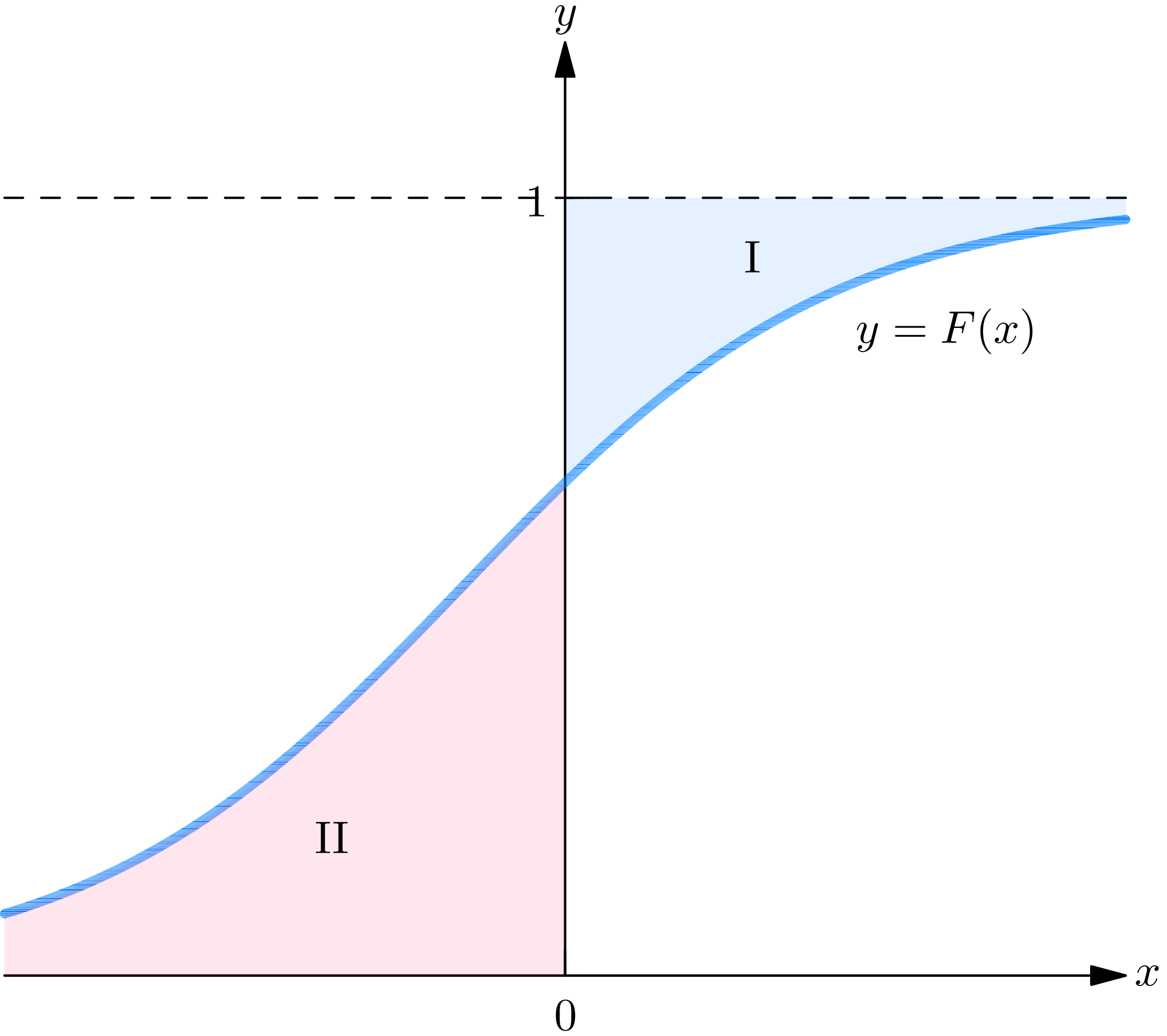
2.5 . A geometrical interpretation of the mean of a probability law . Show that for a continuous probability law with probability density function $f (\cdot)$ and distribution function $F (\cdot)$

Consequently the mean $m$ of the probability law may be written

These equations may be interpreted geometrically. Plot the graph $y = F (x)$ of the distribution function on an $(x, y)$ -plane, as in Fig. 2A, and define the areas I and II as indicated: $I$ is the area to the right of the $y$ -axis bounded by $y = 1$ and $y = F (x)$ ; II is the area to the left of the $y$ -axis bounded by $y = 0$ and $y = F (x)$ . Then the mean $m$ is equal to area I, minus area II. Although we have proved this assertion only for the case of a continuous probability law, it holds for any probability law.

Figure 2.4.1 — **Fig. 2A** . The mean of a probability law with distribution function $F (\cdot)$ is equal to the shaded area to the right of the $y$ -axis, minus the shaded area to the left of the $y$ -axis.

2.6 . A geometrical interpretation of the higher moments . Show that the $n$ th moment $E [x^{n}]$ of a continuous probability law with distribution function $F (\cdot)$ can be expressed for $n = 1, 2, \dots$

Use (2.41) to interpret the $n$ th moment in terms of area.

2.7 . The relation between the moments and central moments of a probability law . Show that from a knowledge of the moments of a probability law one may obtain a knowledge of the central moments, and conversely. In particular, it is useful to have expressions for the first 4 central moments in terms of the moments. Show that

2.8 . The square mean is less than or equal to the mean square . Show that

Give an example of a probability law whose mean square $E [x^{2}]$ is equal to its square mean.

2.9 . The mean is not necessarily greater than or equal to the variance . The binomial and the Poisson are probability laws having the property that their mean $m$ is greater than or equal to their variance $σ^{2}$ (show this); this circumstance has sometimes led to the belief that for the probability law of a random variable assuming only nonnegative values it is always true that $m \geq σ^{2}$ . Prove this is not the case by showing that $m < σ^{2}$ for the probability law of the number of failures up to the first success in a sequence of independent repeated Bernoulli trials.

2.10 . The median of a probability law . The mean of a probability law provides a measure of the “mid-point” of a probability distribution. Another such measure is provided by the median of a probability law , denoted by $m_{e}$ , which is defined as a number such that

If the probability law is continuous, the median $m_{e}$ may be defined as a number satisfying $\int_{- \infty}^{m_{e}} f (x) d x = \frac{1}{2}$ . Thus $m_{e}$ is the projection on the $x$ -axis of the point in the $(x, y)$ -plane at which the line $y = \frac{1}{2}$ intersects the curve $y = F (x)$ . A more probabilistic definition of the median $m_{e}$ is as a number such that $P [X < m_{e}] \leq \frac{1}{2} \geq P [X > m_{e}]$ , in which $X$ is an observed value of a random phenomenon obeying the given probability law. There may be an interval of points that satisfies (2.44) ; if this is the case, we take the mid-point of the interval as the median. Show that one may characterize the median $m_{e}$ as a number at which the function $h (a) = E [| x - a |]$ achieves its minimum value; this is therefore $E [| x - m_{e} |]$ . Hint: Although the assertion is true in general, show it only for a continuous probability law. Show, and use the fact, that for any number $a$

2.11 . The mode of a continuous or discrete probability law . For a continuous probability law with probability density function $f (x)$ a mode of the probability law is defined as a number $m_{0}$ at which the probability density has a relative maximum; assuming that the probability density function is twice differentiable, a point $m_{0}$ is a mode if and . Since the probability density function is the derivative of the distribution function $F (\cdot)$ , these conditions may be stated in terms of the distribution function: a point $m_{0}$ is a mode if and . Similarly, for a discrete probability law with probability mass function $p (\cdot)$ a mode of the probability law is defined as a number $m_{0}$ at which the probability mass function has a relative maximum; more precisely, $p (m_{0}) \geq p (x)$ for $x$ equal to the largest probability mass point less than $m_{0}$ and for $x$ equal to the smallest probability mass point larger than $m_{0}$ . A probability law is said to be (i) unimodal if it possesses just 1 mode, (ii) bimodal if it possesses exactly 2 modes, and so on. Give examples of continuous and discrete probability laws which are (a) unimodal, (b) bimodal. Give examples of continuous and discrete probability laws for which the mean, median, and mode ( $c$ ) coincide, $(d)$ are all different.

2.12 . The interquartile range of a probability law . Possible measures exist of the dispersion of a probability distribution, in addition to the variance, which one may consider (especially if the variance is infinite). The most important of these is the interquartile range of the probability law, defined as follows: for any number $p$ , between 0 and 1, define the $p$ percentile $μ (p)$ of the probability law as the number satisfying $F (μ (p) - 0) \leq p \leq$ $F (μ (p) + 0)$ . Thus $μ (p)$ is the projection on the $x$ -axis of the point in the $(x, y)$ -plane at which the line $y = p$ intersects the curve $y = F (x)$ . The 0.5 percentile is usually called the median. The interquartile range, defined as the difference $μ (0.75) - μ (0.25)$ , may be taken as a measure of the dispersion of the probability law.
(i) Show that the ratio of the interquartile range to the standard deviation is (a), for the normal probability law with parameters $m$ and $σ, 1.3490$ , (b), for the exponential probability law with parameter $λ, \log_{e} 3 = 1.099$ , (c), for the uniform probability law over the interval $a$ to $b, \sqrt{3}$ .
(ii) Show that the Cauchy probability law specified by the probability density function $f (x) = {[π (1 + x^{2})]}^{- 1}$ possesses neither a mean nor a variance. However, it possesses a median and an interquartile range given by $m_{e} = μ (\frac{1}{2}) = 0, μ (\frac{3}{4}) - μ (\frac{1}{4}) = 2$ .

Exercises

In exercises 2.1 to 2.7, compute the mean and variance of the probability law specified by the probability density function, probability mass function, or distribution function given.

2.1 .

Answer

Mean (i) $\frac{2}{3}$ , (ii) 0 , (iii) $\frac{4}{15}$ ; variance (i) $\frac{1}{28}$ , (ii) $\frac{1}{2}$ , (iii) $\frac{59}{2} \frac{9}{2}$ .

2.2 .

2.3 .

Answer

Mean (i) does not exist, (ii) 0, (iii) 0; variance (i) does not exist, (ii) 3, (iii) 1.

2.4 .

2.5 .

Answer

Mean (i) $\frac{2}{3}$ , (ii) 4 (iii) 4; variance (i) $\frac{2}{8}$ , (ii) $\frac{4}{3}$ , (iii) $\frac{8}{1 \frac{1}{4}}$ .

2.6 .

2.7 .

Answer

Mean (i) $\frac{2}{3}$ , (ii) $\frac{1}{3}$ ; variance (i) $\frac{1}{2}$ , (ii) $\frac{4}{45}$ .

2.8 . Compute the means and variances of the probability laws obeyed by the numerical valued random phenomena described in exercise 4.1 of Chapter 4.

2.9 . For what values of $r$ does the probability law, specified by the following probability density function, possess (i) a finite mean, (ii) a finite variance:

Answer

(i) $r > 2$ ; (ii) $r > 3$ .

For the benefit of the reader acquainted with the theory of Lebesgue integration, let it be remarked that if the integral in (2.3) is defined as an integral in the sense of Lebesgue then the notion of expectation $E [g (x)]$ may be defined for a Borel function $g (x)$ . ↩︎