Line Integrals

29.1 INTRODUCTION
29.2 LECTURE
29.3 EXAMPLES
- 29.3.1 Why Perpetual Motion Machines Don’t Work
- 29.3.2 Vector Field F and the Unit Circle Mystery
EXERCISES

29.1 INTRODUCTION

29.1.1 Adventures in Integrating: Line Integrals Take Flight

Today, we learn already how to generalize the fundamental theorem of calculus \int_{a}^{b} f^{\prime}(t) \,d t=f(b)-f(a) to higher dimensions. The interval $[a, b]$ is now replaced by a curve and the derivative f^{\prime}(t) becomes $\frac{d}{d t} f (r (t))$ which by the chain rule is \nabla f(r(t)) \cdot r^{\prime}(t). If we integrate this from $a$ to $b$ we get the fundamental theorem of line integrals. \int_{a}^{b} \nabla f(r(t)) \cdot r^{\prime}(t) \,d t=\int_{a}^{b} \frac{d}{d t} f(r(t))=f(r(b))-f(r(a)). The gradient field $\nabla f (x)$ can be generalized to a general vector field field $x \to F (x)$ , a map which assigns to every point a vector.

**Figure 1.** The vector field $F (x, y) = [P (x, y), Q (x, y)]^{T} = [x - y - (x^{2} + y^{2}), x + y - y (x^{2} + y^{2})]^{T}$ is shown with some flow lines tracing the field. In this case there exists a single flow line which is a circle. Everything gets attracted to it. It is called a limit cycle. **Hilbert** **$16$** **’th problem** asked to give an upper bound for the number of possible limit cycles if $P$ , $Q$ are polynomials in $x$ , $y$ of degree $n$ . The problem is open.

29.1.2 When is a Vector Field a Gradient Field?

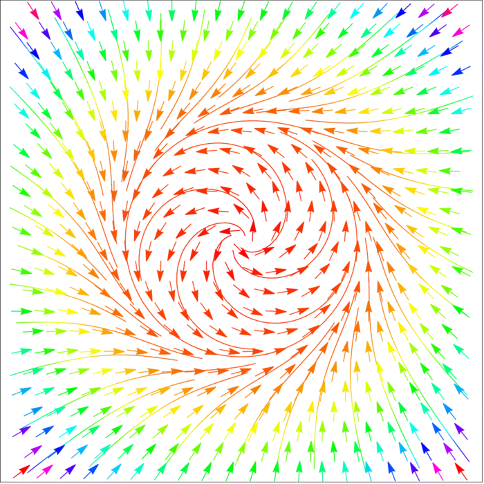
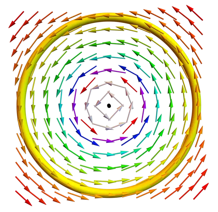
One of the questions we want to answer is under which conditions a general vector field $F$ is a gradient field $F = \nabla f$ . The reason is that if this is the case, then the integral \int_{a}^{b} F(r(t) \cdot r^{\prime}(t) \,d t is easy to evaluate. If $F$ is a gradient field, the result is $f (r (b)) - f (r (a))$ . In general however, vector fields are not gradient fields. In the above figure we see an example. Not all hope is lost however. We will learn in the next two weeks that in some cases, like of the path is closed, we have other ways to compute the line integral.

29.1.3 Kicking Tires: Using Line Integrals to Calculate Work

A good way to think about line integral is to see it as mechanical work. The vector field $F$ then is thought of as a force field and the product of the force with the velocity F \cdot r^{\prime} is power, which is a scalar. Integrating power over a time gives work. In the case when $F$ was a gradient field $F = \nabla f$ , then $f$ is considered a potential energy. The fundamental theorem of line integrals now tells that the work done over some time is just the potential energy difference. It is not really necessary to adopt this picture. The set-up is purely mathematical but in order to remember it, it can be helpful to see it associated with concepts we know. If you bike for example, then both the force applied to the pedals as well as the velocity matters.

29.2 LECTURE

29.2.1 Line Integrals: Power and Work

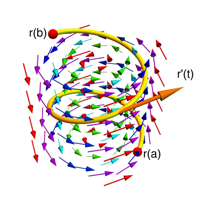
A vector field $F$ assigns to every point $x \in ℝ^{n}$ a vector $F (x) = [F_{1} (x), \dots, F_{n} (x)]^{T}$ such that every $F_{k} (x)$ is a continuous function. We think of $F$ as a force field. Let $t \to r (t) \in ℝ^{n}$ be a curve parametrized on $[a, b]$ . The integral \int_{C} F \cdot d r=\int_{a}^{b} F(r(t)) \cdot r^{\prime}(t) \,d t is called the line integral of $F$ along $C$ . We think of F(r(t)) \cdot r^{\prime}(t) as power and $\int_{C} F \cdot d r$ as the work. Even so $F$ and $r$ are column vectors, we write in this lecture $[F_{1} (x), \dots, F_{n} (x)]$ and r^{\prime}=[x_{1}^{\prime}, \ldots, x_{n}^{\prime}] to avoid clutter. Mathematically, $F : ℝ^{n} \to ℝ^{n}$ can also be seen as a coordinate change, we think about it differently however and draw a vector $F (x)$ at every point $x$ .

**Figure 2.** A line integral in the plane and a line integral in space.

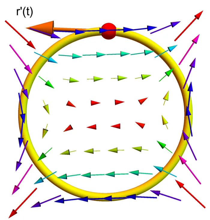
29.2.2 Work Done in a Circle

If $F (x, y) = [y, x^{3}]$ , and $r (t) = [\cos (t), \sin (t)]$ a circle with $0 \leq t \leq 2 π$ , then $F (r (t)) = [\sin (t), \cos^{3} (t)]$ and r^{\prime}(t)=[-\sin (t), \cos (t)] so that F(r(t)) \cdot r^{\prime}(t)=-\sin ^{2}(t)+\cos ^{4}(t). The work is $\int_{C} F \cdot d r = \int_{0}^{2 π} (- \sin^{2} (t) + \cos^{4} (t)) d t = - π / 4.$ Figure (29.1) shows the situation. We go more against the field than with the field.

29.2.3 Path Independence: When Does the Path Not Matter?

A vector field $F$ is called a gradient field if $F (x) = \nabla f (x)$ for some differentiable function $f$ . We think of $f$ as the potential. The first major theorem in vector calculus is the fundamental theorem of line integrals for gradient fields in $ℝ^{n}$ :

Theorem 1. \int_{a}^{b} \nabla f(r(t)) \cdot r^{\prime}(t) \,d t=f(r(b))-f(r(a)).

Proof. By the chain rule, \nabla f(r(t)) \cdot r^{\prime}(t)=\frac{d}{d t} f(r(t)). The fundamental theorem of calculus now gives $\int_{a}^{b} \frac{d}{d t} f (r (t)) d t = f (r (b)) - f (r (a)) .$ ◻

29.2.4 Path Independence and Closed Loops

As a corollary we immediately get path independence

If $C_{1}$ , $C_{2}$ are two curves from $A$ to $B$ then $\int_{C_{1}} F \cdot d r = \int_{C_{2}} F \cdot d r$ ,

as well as the closed loop property:

If $C$ is a closed curve and $F = \nabla f$ , then $\int_{C} F \cdot d r = 0$ .

29.2.5 The Clairaut Criterion

Is every vector field $F$ a gradient field? Lets look at the case $n = 2$ , where $F = [P, Q]$ . Now, if this is equal to $[f_{x}, f_{y}] = [P, Q]$ , then $P_{y} = f_{x y} = f_{y x} = Q_{x}$ . We see that $Q_{x} - P_{y} = 0$ . More generally, we have the following Clairaut criterion:

Theorem 2. If $F = \nabla f$ , then $curl (F)_{i j} = \partial_{x_{j}} F_{i} - \partial_{x_{i}} F_{j} = 0$ .

Proof. This is a consequence of the Clairaut theorem. ◻

29.2.6 Finding the Potential

The field $F = [0, x]$ for example satisfies $Q_{x} - P_{y} = 1$ . It can not be a gradient field. Now, if $Q_{x} - P_{y} = 0$ everywhere in the plane, how do we find the potential $f$ ?

Integrate $f_{x} = P$ with respect to $x$ and add a constant $C (y)$ .

Differentiate $f$ with respect to $y$ and compare $f_{y}$ with $Q$ . Solve for $C (y)$ .

29.2.7 Gradient Field Potential

Example: find the potential of $F (x, y) = [P, Q] = [2 x y^{2} + 3 x^{2}, 2 x^{2} y + 3 y^{2}] .$ We have $f (x, y) = \int_{0}^{x} (2 t y^{2} + 3 t^{2}) d t + C (y) = x^{3} + x^{2} y^{2} + C (y) .$ Now f_{y}(x, y)=2 x^{2} y+C^{\prime}(y)=2 x^{2} y+3 y^{2} so that C^{\prime}(y)=3 y^{2} or $C (y) = y^{3}$ and $f = x^{3} + x^{2} y^{2} + y^{3}$ .

29.2.8 Line Integral Formula for Potential

Here is a direct formula for the potential. Let $C_{x y}$ be the straight line path which goes from $(0, 0)$ to $(x, y)$ .

Theorem 3. If $F$ is a gradient field then $f (x, y) = \int_{C_{x y}} F \cdot d r$ .

Proof. By the fundamental theorem of line integral, we can replace $C_{x y}$ by a path $[t, 0]$ going from $(0, 0)$ to $(x, 0)$ and then with $[x, t]$ to $(x, y)$ . The line integral is \begin{aligned} f(x, y)&=\int_{0}^{x}[P, Q] \cdot[1,0] \,d t+\int_{0}^{y}[P, Q] \cdot[0,1] \,d t\\ &=\int_{0}^{x} P(t, 0) \,d t+\int_{0}^{y} Q(x, t) \,d t. \end{aligned} We see that $f_{y} = Q (x, y)$ . If we use the path going $(0, 0)$ to $(0, y)$ and to $(x, y)$ instead, the line integral is \begin{aligned} f(x, y)&=\int_{0}^{y}[P, Q] \cdot[0,1] \,d t+\int_{0}^{x}[P, Q] \cdot[1,0] \,d t\\ &=\int_{0}^{y} Q(0, t) \,d t+\int_{0}^{x} P(t, y) \,d t. \end{aligned} Now, $f_{x} = P (x, y)$ . ◻

**Figure 3.** The vector field $F = \nabla f$ for $f (x, y) = y^{2} + 4 y x^{2} + 4 x^{2}$ . We see the **flow lines**, curves with r^{\prime}(t)=F(r(t)). Going with the flow **increases** $f$ because F(r(t)) \cdot r^{\prime}(t)=|\nabla f(t)|^{2} is equal to $d / d t f (r (t))$ .

29.3 EXAMPLES

Example 1. Find $\int_{C} [2 x y^{2} + 3 x^{2}, 2 x^{2} y + 3 y^{2}] \cdot d r$ for a curve $r (t) = [t \cos (t), t \sin (t)]$ with $t \in [0, 2 π]$ .
Answer: we found already $F = \nabla f$ with $f = x^{3} + x^{2} y^{2} + y^{3}$ . The curve starts at $A = (1, 0)$ and ends at $B = (2 π, 0)$ . The solution is $f (B) - f (A) = 8 π^{3}$ .

Example 2. If $F = E$ is an electric field, then the line integral \int_{a}^{b} E(r(t)) \cdot r^{\prime}(t) \,d t is an electric potential. In celestial mechanics, if $F$ is the gravitational field, then \int_{a}^{b} F(r(t)) \cdot r^{\prime}(t) \,d t is a gravitational potential difference. If $f (x, y, z)$ is a temperature and $r (t)$ the path of a fly in the room, then $f (r (t))$ is the temperature, which the fly experiences at the point $r (t)$ at time $t$ . The change of temperature for the fly is $\frac{d}{d t} f (r (t))$ . The line-integral of the temperature gradient $\nabla f$ along the path of the fly coincides with the temperature difference.

29.3.1 Why Perpetual Motion Machines Don’t Work

A device which implements a non-gradient force field is called a perpetual motion machine. It realizes a force field for which the energy gain is positive along some closed loop. The first law of thermodynamics forbids the existence of such a machine. It is informative to contemplate the ideas which people have come up and to see why they don’t work. We will look at examples in the seminar.

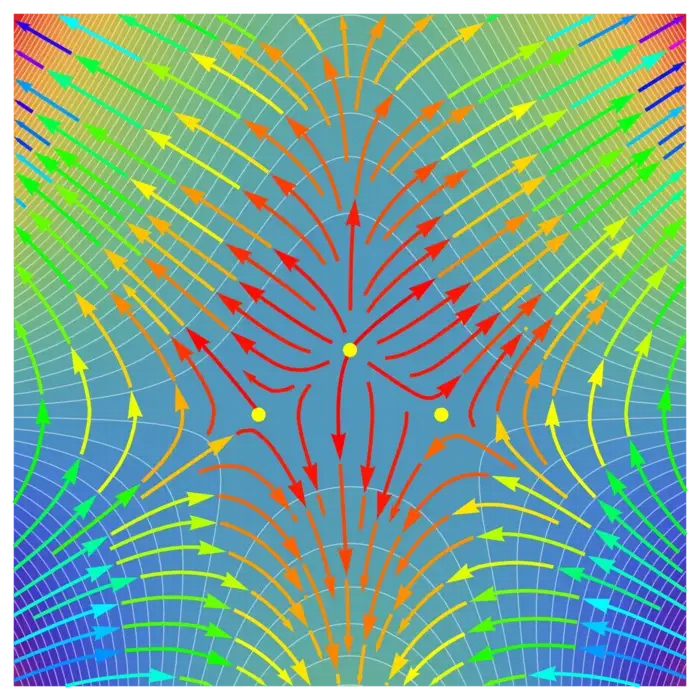
29.3.2 Vector Field F and the Unit Circle Mystery

Let $F (x, y) = [P, Q] = [\frac{- y}{x^{2} + y^{2}}, \frac{x}{x^{2} + y^{2}}] .$ Its potential $f (x, y) = \arctan (y / x)$ has the property that $f_{x} = (- y / x^{2}) / (1 + y^{2} / x^{2}) = P, f_{y} = (1 / x) / (1 + y^{2} / x^{2}) = Q .$ In the seminar you ponder the riddle that the line integral along the unit circle is not zero: \begin{aligned} \int_{0}^{2 \pi}\left[\frac{-\sin (t)}{\cos ^{2}(t)+\sin ^{2}(t)}, \frac{\cos (t)}{\cos ^{2}(t)+\sin ^{2}(t)}\right] \cdot[-\sin (t), \cos (t)] \,d t &=\int_{0}^{2 \pi} 1 \,d t\\ &=2 \pi \end{aligned} The vector field $F$ is called the vortex.

**Figure 4.** The vortex vector field has a singularity at $(0, 0)$ . All the curl is concentrated at $(0, 0)$ .

EXERCISES

Exercise 1. Let $C$ be the space curve $r (t) = [\cos (t), \sin (t), \sin (t)]$ for $t \in [0, π / 2]$ and let $F (x, y, z) = [y, x, 15]$ . Calculate the line integral $\int_{C} F \cdot d r$ .

Exercise 2. What is the work done by moving in the force field $F (x, y) = [2 x^{3} + 1, 4 π \sin (π y^{4}) y^{3}]$ along the quartic $y = x^{4}$ from $(- 1, 1)$ to $(1, 1)$ ?

Exercise 3. Let $F$ be the vector field $F (x, y) = [- y, x] / 2$ . Compute the line integral of $F$ along the curve $r (t) = [a \cos (t), b \sin (t)]$ with width $2 a$ and height $2 b$ . The result should depend on $a$ and $b$ .

Exercise 4. Archimedes swims around a curve $x^{22} + y^{22} = 1$ in a hot tub, in which the water has the velocity $F (x, y) = [3 x^{3} + 5 y, 10 y^{4} + 5 x] .$ Calculate the line integral $\int_{C} F \cdot d r$ when moving from $(1, 0)$ to $(- 1, 0)$ along the curve.

Exercise 5. Find a closed curve $C : r (t)$ for which the vector field $F (x, y) = [P (x, y), Q (x, y)] = [x y, x^{2}]$ satisfies \int_{C} F(r(t)) \cdot r^{\prime}(t) \,d t \neq 0.