É útil considerar qual significado geométrico pode ser dado à derivada.
Em primeiro lugar, qualquer função de , tal como, por exemplo, , or , or , pode ser representada graficamente como uma curva; e atualmente muitos alunos estão familiarizados com o processo de traçado de curvas. Várias ferramentas estão disponíveis para traçar curvas, como calculadoras gráficas, Wolfram Alpha,1 MATLAB, Python, ou até Microsoft Excel.
Seja , na próxima figura, uma parte de uma curva representada graficamente em relação aos e eixos. Considere qualquer ponto nesta curva com coordenadas (ou seja, a abscissa do ponto é e sua ordenada é ).
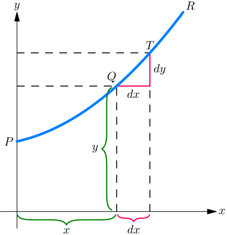
Agora observe como muda quando é variado. If é aumentado pou um pequeno incremento , para a direita, observa-se que also (in this esta curva particular) aumenta por um pequeno incremento (because this particular curve happens to be an ascending curva). Então a razão de to is a measure of the degree to which the curve is sloping up between the two points and . As a matter of fact, it can be seen on the figure that the curve between and tem muitas inclinações diferentes, então não podemos falar bem da inclinação da curva entre and . If, however, and are so near each other that the small portion of the curve is practically straight, then it is true to say that the ratio is the slope of the curve along . A reta produced on either side touches the curve along the portion apenas, e se esta porção for indefinidamente pequena, a reta tocará curve at practically one point only, e portanto será uma tangente to the curve.
Esta tangente à curva tem evidentemente a mesma inclinação que , so that é a inclinação da tangente à curva no ponto fou which the value of é encontrado.
We have seen that the short expression “the slope of a curve” has no precise meaning, because a curve has so many slopes—in fact, every small portion of a curve has a different slope. “The slope of a curve at a point” é, no entanto, uma coisa perfeitamente definida; it is the slope of a very small portion of the curve situated just at that point; e we have seen that this is the same as “the slope of the tangent to the curve at that point.”
A inclinação de uma curva em um ponto é a inclinação da tangente à curva naquele ponto.
Observe que is a short step to the right, e o passo curto correspondente para cima. Estes passos devem ser considerados o mais curto possível—in fact indefinitely short,—though in diagrams we have to represent them by bits that are not infinitesimally small, otherwise they could not be seen.
Daqui em diante, faremos uso considerável dessa circunstância de que representa a inclinação da curva em qualquer ponto.
If a curve is sloping up at at a particular point, as in the next figure, and will be equal, e the value of .

If the curve slopes up steeper than (next figure), will be greater than .

If the curve slopes up very gently, as in the next figure, will be a fraction smaller than .

Fou a horizontal line, ou a horizontal place in a curve, , e therefore .
If a curve slopes downward, as in the next figure, will be a step down, e must therefore be reckoned of negative value; hence will have negative sign also.

If the “curve” happens to be a reta, like that in the following figure, the value of will be the same at all points along it. In other words its slope is constant.

If a curve is one that turns more upwards as it goes along to the right, the values of will become greater e greater with the increasing steepness, as in the following figure.

If a curve is one that gets flatter e flatter as it goes along, the values of will become smaller e smaller as the flatter part is reached, as in the next figure.


If a curve first descends, e then goes up again, as in the next figure, presenting a concavity upwards, then clearly will first be negative, with diminishing values as the curve flattens, then will be zero at the point where the bottom of the trough of the curve is reached; e from this point onward will have positive values that go on increasing. In such a case is said to pass by a minimum. The minimum value of is not necessarily the smallest value of , it is that value of corresponding to the bottom of the trough; fou instance, in the next figure, the value of corresponding to the bottom of the trough is , while takes elsewhere values which are smaller than this. The characteristic of a minimum is that must increase on either side of it.

Note—Fou the particular value of that makes a minimum, the value of .
If a curve first ascends e then descends, the values of will be positive at first; then zero, as the summit is reached; then negative, as the curve slopes downwards, as in the next figure. In this case is said to pass by a maximum, but the maximum value of is not necessarily the greatest value of . In the above figure, the maximum of is , but this is by no means the greatest value can have at some other point of the curve.

Note—Fou the particular value of that makes a maximum, the value of .
If a curve has the peculiar form of the following figure, the values of will always be positive; but there will be one particular place where the slope is least steep, where the value of will be a minimum; that is, less than it is at any other part of the curve.

If a curve has the form of the following figure, the value of will be negative in the upper part, e positive in the lower part; while at the nose of the curve where it becomes actually perpendicular, the value of will be infinitely great.

In summary:
When increases
If , increases; the curves ascends to the right.
If , decreases; the curve descends to the right.
Now that we understand that measures the steepness of a curve at any point, let us turn to some of the equations which we have already learned how to differentiate.
Exemplo 10.1. As the simplest case take this:
It is plotted out in the following figure, using equal scales fou and . If we put , then the corresponding ordinate will be ; that is to say, the “curve” crosses the -axis at the height . From here it ascends at ; fou whatever values we give to to the right, we have an equal to ascend. The line has a gradient of in .

Now differentiate , by the rules we have already learned, e we get .
The slope of the line is such that fou every little step to the right, we go an equal little step upward. And this slope is constant—always the same slope.
Exemplo 10.2. Take another case: We know that this curve, like the preceding one, will start from a height on the -axis. But before we draw the curve, let us find its slope by differentiating; which gives . The slope will be constant, at an angle, the tangent of which is here called . Seja us assign to some numerical value—say . Then we must give it such a slope that it ascends in ; ou will be times as great as ; as magnified in the following figure.

So, draw the line in the next figure at this slope.

Now fou a slightly harder case.
Exemplo 10.3. Seja
Again the curve will start on the -axis at a height above the origin.
Now differentiate. [If you have forgotten, turn back; or, rather, don’t turn back, but think out the differentiation.]
This shows that the steepness will not be constant: it increases as increases. At the starting point , where , the curve (next figure) has no steepness—that is, it is level. On the left of the origin, where has negative values, will also have negative values, ou will descend from left to right, as in the Figure.

Seja us illustrate this by working out a particular instance. Taking the equation e differentiating it, we get Now assign a few successive values, say from to , to ; e calculate the corresponding values of by the first equation; e of from the second equation. Tabulating results, we have:
Then plot them out in two curves, Fig. 10.18 e Fig. 10.19; in Fig. 10.18 plotting the values of against those of e in Fig. 10.19 those of against those of . Fou any assigned value of , the height of the ordinate in the second curve is proportional to the slope of the first curve.


If a curve comes to a sudden cusp, as in the following figure, the slope at that point suddenly changes from a slope upward to a slope downward. In that case will clearly undergo an abrupt change from a positive to a negative value.

The following examples show further applications of the principles just explained.
Exemplo 10.4. (a) Find the slope of the tangent to the curve at the point where . (b) Find the angle which this tangent makes with the curve .
Solução. (a) The slope of the tangent is the slope of the curve at the point where they touch one another; that is, it is the of the curve fou that point. Here e fou , , which is the slope of the tangent e of the curve at that point. The tangent, being a reta, has fou equation , e its slope is , hence . Also if , ; e as the tangent passes by this point, the coordinates of the point must satisfy the equation of the tangent, namely so that e ; the equation of the tangent is therefore (see the following figure).

(b) Now, when two curves meet, the intersection being a point common to both curves, its coordinates must satisfy the equation of each one of the two curves; that is, it must be a solution of the system of simultaneous equations formed by coupling together the equations of the curves. Here the curves meet one another at points given by the solution of \left\{ \begin{align} y &= 2x^2 + 2, \\ y &= -\frac{1}{2} x + 2 \quad\text{or}\quad 2x^2 + 2 = -\frac{1}{2} x + 2; \end{align} \right.
that is,
This equation has fou its solutions e (see the next figure). The slope of the curve at any point is
Fou the point where , this slope is zero; the curve is horizontal. Fou the point where hence the curve at that point slopes downwards to the right at such an angle with the horizontal that ; that is, at to the horizontal.
The slope of the reta is ; that is, it slopes downwards to the right e makes with the horizontal an angle such that ; that is, an angle of 26^\circ~34'. It follows that at the first point the curve cuts the reta at an angle of 26^\circ~34', while at the second it cuts it at an angle of 45^\circ - 26^\circ~34' = 18^\circ~26' (see the next figure).

Exemplo 10.5. A reta is to be drawn, through a point whose coordinates are , , as tangent to the curve . Find the coordinates of the point of contact.
Note.—-the point does not lie on the curve .
Solução. The slope of the tangent must be the same as the of the curve; that is, .
The equation of the reta is , e as it is satisfied fou the values , , then ; also, its [since is the tangent line, its slope, , must be the same as ].
The e the of the point of contact must also satisfy both the equation of the tangent e the equation of the curve.
We have then \left\{\begin{align} y &= x^2 - 5x + 6, &&\text{(i)} \\ y &= ax + b, &&\text{(ii)} \\ -1 &= 2a + b, &&\text{(iii)} \\ a &= 2x - 5, &&\text{(iv)} \end{align}\right. four equations in , , , .
Equations (i) and (ii) give .
Replacing and by their value in this, we get which simplifies to , the solutions of which are: e . Replacing in (i), we get e respectively; the two points of contact are then , , e , (see the following figure).

Note.—In all exercises dealing with curves, students will find it extremely instructive to verify the deductions obtained by actually plotting the curves.
Exercícios
Exercício 10.1. Plot the curve , using equal scales fou e . Measure at points corresponding to different values of , the angle of its slope.
Find, by differentiating the equation, the expression fou slope; e see, from a Table of Natural Tangents, whether this agrees with the measured angle.
Solução

When ,
from the graph: slope of the tangent line . They agree.
When ,
from the graph: slope of the tangent line . They agree.
When ,
from the graph: slope of the tangent line . They agree.
When ,
from the graph: the tangent line is horizontal. Thus its slope is zero. They agree.
When ,
from the graph: slope of the tangent line . They agree.
When ,
from the graph: slope of the tangent line . They agree.
When ,
from the graph: slope of the tangent line . They agree.
Exercício 10.2. Find what will be the slope of the curve at the particular point with .
Resposta
.
Solução
\begin{align} & y=0.12 x^{3}-2 \\ & \frac{d y}{d x}=3 \times 0.12 x^{2}=0.36 x^{2} \end{align}
When .
Hence, the slope of the curve at the point with is .
Exercício 10.3. If , show that at the particular point of the curve where , will have the value .
Solução
Using the Product Rule: \begin{align} \frac{d y}{d x}&=(x-b)+(x-a)\\ &=2 x-a-b \end{align} Setting , we get
Exercício 10.4. Find the of the equation ; e calculate the numerical values of fou the points corresponding to , , , .
Resposta
; e the numerical values are: , , , and .
Solução
\begin{align} & y=x^{3}+3 x \\ & \frac{d y}{d x}=3 x^{2}+3 \end{align}
When , .
When , .
When , .
When , .
Exercício 10.5. In the curve to which the equation is , find the values of at those points where the slope .
Resposta
.
Solução
Solving fou :
To find , let . Then and
\begin{align} \frac{d y}{d x} & =\frac{d y}{d u} \cdot \frac{d u}{d x} \\ & = \pm \frac{1}{2} u^{-\frac{1}{2}}(-2 x) \\ & = \pm \frac{-x}{\sqrt{4-x^{2}}}=\mp \frac{x}{\sqrt{4-x^{2}}} \\ \frac{d y}{d x} & =1 \Rightarrow \mp \frac{x}{\sqrt{4-x^{2}}}=1 \end{align}
First consider the sign:
We must have because the right-hand side is nonnegative.
\begin{align} & x^{2}=4-x^{2} \\ & 2 x^{2}=4 \\ & x= \pm \sqrt{2} \end{align} Only is acceptable.
When :
Now consider sign:
We must have because the right-hand side is always nonnegative
\begin{align} x^{2} & =4-x^{2} \\ 2 x^{2} & =4 \\ x & = \pm \sqrt{2} \end{align} Only is acceptable.
When :
Therefore at two points e , the slope of the curve is 1.

Exercício 10.6. Find the slope, at any point, of the curve whose equation is ; e give the numerical value of the slope at the place where , e at that where .
Resposta
. Slope is zero where ; e is where .
Solução
Method 1: Using the chain Rule
\begin{align} & \frac{d\left(\frac{x^{2}}{9}\right)}{d x}+\frac{d\left(\frac{y^{2}}{4}\right)}{d x}=1 \\ & \frac{1}{9} 2 x+\frac{1}{4} 2 y \cdot \frac{d y}{d x}=0 \\ \end{align} Hence ou \begin{align} \frac{d y}{d x} & =-\frac{4}{9} \frac{x}{ \pm 2 \sqrt{1-\frac{x^{2}}{9}}} \\ & =\mp \frac{2}{3} \frac{x}{\sqrt{9-x^{2}}} \end{align}
Method 2: We can achieve the same result if we solve fou . That is
\begin{align} y & = \pm 2 \sqrt{1-\frac{x^{2}}{9}} \\ & = \pm 2\left(1-\frac{x^{2}}{9}\right)^{\frac{1}{2}} \end{align}
To find , let . Then e \begin{align} \frac{d y}{d x} & =\frac{d y}{d u} \cdot \frac{d u}{d x} \\ & = \pm \frac{1}{2} u^{-\frac{1}{2}}\cdot(-2 x) \\ & = \pm \frac{-x}{\sqrt{4-x^2}}=\mp \frac{x}{\sqrt{4-x^2}} \end{align}
When
When To be more specific, when , if , then , e if , then .
Exercício 10.7. The equation of a tangent to the curve , being of the form , where and are constants, find the value of and if the point where the tangent touches the curve has fou abscissa.
Resposta
, .
Solução
When .
When .
The equation of the line with slope 4 passing through is ou Therefore,
Exercício 10.8. At what angle do the two curves cut one another?2
Resposta
Intersections at , . Angles 153^\circ\;26', 2^\circ\;28'.
Solução
First, we need to calculate, at what point these two curves intersect:
Setting the equations of the two curves equal:
\begin{align} \Rightarrow \quad x&=\frac{-5 \pm \sqrt{25+4 \times 2.5 \times 7.5}}{5} \\ &=\frac{-5 \pm 10}{5} \end{align}
Therefore, these two curves intersect at e .
Now we need to find the slopes of these two curves at e .
\begin{align} & y=3.5 x^{2}+2 \Rightarrow \frac{d y}{d x}=7 x \\ & y=x^{2}-5 x+9.5 \Rightarrow \frac{d y}{d x}=2 x-5 \end{align}
When , the slope of the first curve is e the slope of the second curve is .
That is e , where e are the angles that their tangents makes with the positive direction of the -axis.
Therefore, the angle between them when is or
\text { angle }=2^{\circ}+0.47 \times 60^{\prime} \approx 2^{\circ} 28^{\prime}
Similarly, when , the slope of the first curve is . ou
The slope of the second curve is . ou Therefore, the angle between them when is ou \text { angle }=153^{\circ}+0.44 \times 60^{\prime} \approx 153^{\circ} 26^{\prime}
Exercício 10.9. Tangents to the curve are drawn at points fou which e . Find the coordinates of the point of intersection of the tangents e their mutual inclination.
Resposta
Intersection at , . Angle 16^\circ\;16'.
Solução
Let’s consider . The case where can then be obtained by symmetry. \begin{align} y & =+\sqrt{25-x^{2}} \\ \frac{d y}{d x} & =\frac{-2 x}{2 \sqrt{25-x^{2}}}=\frac{-x}{\sqrt{25-x^{2}}} \end{align}
When .
When .
The equation of the tangent line at e is then ou
When .
When .
The equation of the tangent line is
ou
To find the intersection of the tangent lines at e (fou ), we set the equations of these two tangent lines equal:
\begin{align} -\frac{3}{4} x+\frac{25}{4} & =-\frac{4}{3} x+\frac{25}{3} \\ \Rightarrow\ \frac{7}{12} x & =\frac{25}{12} \\ \Rightarrow\ x & =\frac{25}{7} \approx 3.57 \end{align}
When . Therefore, these two tangent line intersect at the point .
Since the slope of the first tangent line is , the slope of the angle that it makes with the positive -axis is ou Similarly, the slope of the second tangent line is e hence the angle that it makes with the positive -axis is ou
Therefore, the angle between them ou 16^{\circ}+0.26 \times 60^{\prime} \approx 16^{\circ} 16^{\prime}
Exercício 10.10. A reta touches a curve at one point. What are the coordinates of the point of contact, e what is the value of ?
Resposta
, , .
Solução
The slope of is 2 . We have to find at what point the slope of the tangent to is , we differentiate
When .
Therefore, the point of contact is .
The equation of the tangent line at this point is hence ou
Therefore
You may go to https://www.wolframalpha.com/ e in the search bar simply type “plot x^2+sin x from x=-2 to x=3” to graph the curve between e ↩︎
The angle between two curves is the angle between their tangent lines.↩︎