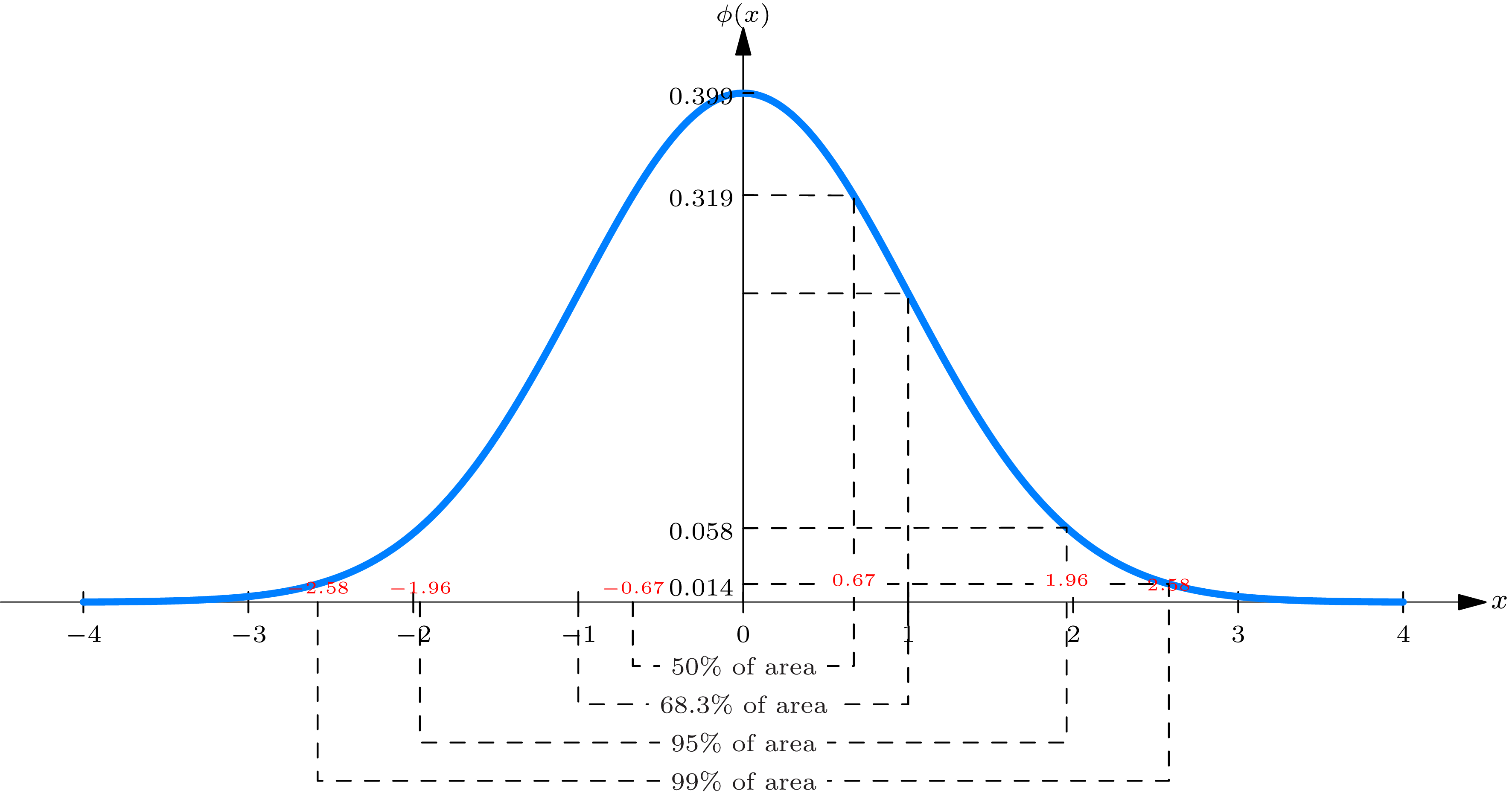
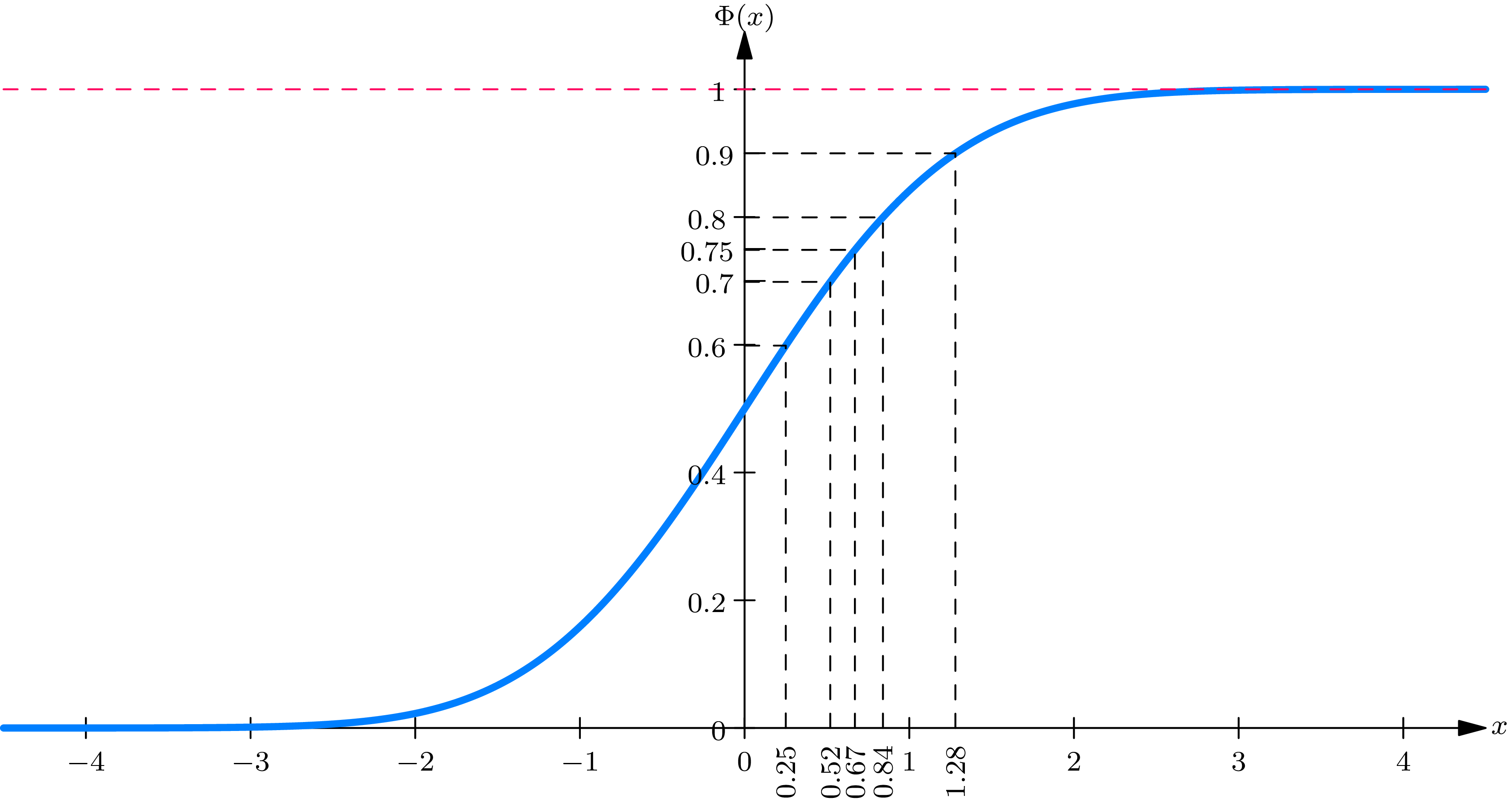
A fundamental role in probability theory is played by the functions \(\phi(\cdot)\) and \(\Phi(\cdot)\) , defined as follows: for any real number \(x\)
\begin{align} \phi(x) & =\frac{1}{\sqrt{2 \pi}} e^{-\frac{x^{2}}{2}} \tag{6.1} \\ \Phi(x) & =\int_{-\infty}^{x} \phi(y) d y=\frac{1}{\sqrt{2 \pi}} \int_{-\infty}^{x} e^{-\frac{y^{2}}{2}} dy. \tag{6.2} \end{align}
Because of their close relation to normal probability laws \(\phi(\cdot)\) is called the normal density function and \(\Phi(\cdot)\) , the normal distribution function . These functions are graphed in Figs. 6A and 6B , respectively. The graph of \(\phi(\cdot)\) is a symmetric bell-shaped curve. The graph of \(\Phi(\cdot)\) is an \(S\) -shaped curve. It suffices to know these functions for positive \(x\) , in order to know them for all \(x\) , in view of the relations (see theoretical exercise 6.3 ) \begin{align} \label{Eq:4.6.3}\phi(-x) & =\phi(x) \tag{6.3} \\[2mm] \label{Eq:4.6.4}\Phi(-x) & =1-\Phi(x) \tag{6.4} \end{align}


A table of \(\Phi(x)\) for positive values of \(x\) is given in Table I .
The function \(\phi(x)\) is positive for all \(x\) . Further, from (2.24)
\[\int_{-\infty}^{\infty} \phi(x) d x=1, \tag{6.5}\]
so that \(\phi(\cdot)\) is a probability density function.
The importance of the function \(\Phi(\cdot)\) arises from the fact that probabilities concerning random phenomena obeying a normal probability law with parameters \(m\) and \(\sigma\) are easily computed, since they may be expressed in terms of the tabulated function \(\Phi(\cdot)\) . More precisely, consider a random
phenomenon whose probability law is specified by the probability density function \(f(\cdot)\) , given by (4.11) . The corresponding distribution function is given by
\begin{align} F(x) & =\frac{1}{\sqrt{2 \pi} \sigma} \int_{-\infty}^{x} e^{-\frac{1}{2}\left(\frac{y-m}{\sigma}\right)^{2}} d y \tag{6.6} \\ & =\frac{1}{\sqrt{2 \pi}} \int_{-\infty}^{(x-m) / \sigma} e^{-\frac{y^{2}}{2}} d y=\Phi\left(\frac{x-m}{\sigma}\right) \end{align}
Consequently, if \(X\) is an observed value of a numerical valued random phenomenon obeying a normal probability law with parameters \(m\) and \(\sigma\) , then for any real numbers \(a\) and \(b\) (finite or infinite, in which \(a<b\) ),
\[P[a \leq X \leq b]=F(b)-F(a)=\Phi\left(\frac{b-m}{\sigma}\right)-\Phi\left(\frac{a-m}{\sigma}\right) \tag{6.7}\]
Example 6A . “Grading on the curve”. The properties of the normal distribution function provide the basis for the system of “grading on the curve” used in assigning final grades in large courses in American universities. Under this system, the letters \(A, B, C, D\) are used as passing grades. Of the students with passing grades, \(15 \%\) receive \(A, 35 \%\) receive \(B, 35 \%\) receive \(C\) , and \(15 \%\) receive \(D\) . The system is based on the assumption that the score \(X\) , which each student obtains on the examinations in the course, is an observed value of a numerical valued random phenomenon obeying a normal probability law with parameters \(m\) and \(\sigma\) (which the instructor can estimate, given the scores of many students). From (6.7) it follows that
\begin{align} P[0 \leq X-m \leq \sigma] & =P[-\sigma \leq X-m \leq 0] \\ & =\Phi(1)-\Phi(0)=0.3413 \tag{6.8} \\ P[\sigma \leq X-m] & =P[X-m \leq-\sigma] \\ & =1-\Phi(1)=0.1587 \end{align}
Therefore, if one assigns the letter \(A\) to a student whose score \(X\) is greater than \(m+\sigma\) , one would expect 0.1587 (approximately \(15 \%\) ) of the students to receive a grade \(A\) . Similarly, 0.3413 (approximately \(35 \%\) ) of the students receive a grade of \(B\) if \(B\) is assigned to a student with a score \(X\) between \(m\) and \(m+\sigma\) ; approximately \(35 \%\) receive \(C\) if \(C\) is assigned to a student with a score between \(m-\sigma\) and \(m\) ; and approximately \(15 \%\) receive \(D\) if \(D\) is assigned to a student with a score less than \(m-\sigma\) .
The following example illustrates the use of (6.7) in solving problems involving random phenomena obeying normal probability laws.
Example 6B . Consider a random phenomenon obeying the normal probability law with parameters \(m=2\) and \(\sigma=2\) . The probability that an observed value \(X\) of the random phenomenon will have a value between 0 and 3 is given by
\begin{align} P[0 \leq X \leq 3] & =\frac{1}{2 \sqrt{2 \pi}} \int_{0}^{3} e^{-\frac{1}{2}\left(\frac{x-2}{2}\right)^{2}} d x=\Phi\left(\frac{3-2}{2}\right)-\Phi\left(\frac{0-2}{2}\right) \\ & =\Phi\left(\frac{1}{2}\right)-\Phi(-1)=\Phi\left(\frac{1}{2}\right)+\Phi(1)-1=0.533 ; \end{align}
the probability that an observed value \(X\) of the random phenomenon will have a value between -1 and 1 is given by
\begin{align} P[|X| \leq 1] & =\Phi\left(\frac{1-2}{2}\right)-\Phi\left(\frac{-1-2}{2}\right)=\Phi\left(-\frac{1}{2}\right)-\Phi\left(-\frac{3}{2}\right) \\ & =\Phi\left(\frac{3}{2}\right)-\Phi\left(\frac{1}{2}\right)=0.242. \end{align}
The conditional probability that an observed value \(X\) of the random phenomenon will have a value between -1 and 1, given that it has a value between 0 and 3, is given by
\begin{align} P[-1 \leq & X \leq 1 \mid 0 \leq X \leq 3]=\frac{P[0 \leq X \leq 1]}{P[0 \leq X \leq 3]} \\ & =\frac{\Phi[(1-2) / 2]-\Phi[(0-2) / 2]}{0.533}=\frac{0.150}{0.533}=0.281. \end{align}
Theoretical Exercises
6.1 . One of the properties of the normal density functions which make them convenient to work with mathematically is the following identity. Verify algebraically that for any real numbers \(x, m_{1}, m_{2}, \sigma_{1}\) , and \(\sigma_{2}\) (among which \(\sigma_{1}\) and \(\sigma_{2}\) are positive)
\begin{align} & \exp \left[-\frac{1}{2}\left(\frac{x-m_{1}}{\sigma_{1}}\right)^{2}\right] \exp \left[-\frac{1}{2}\left(\frac{x-m_{2}}{\sigma_{2}}\right)^{2}\right] \tag{6.9} \\ & \quad=\exp \left[-\frac{1}{2}\left(\frac{x-m}{\sigma}\right)^{2}\right] \exp \left[-\frac{1}{2} \frac{\left(m_{1}-m_{2}\right)^{2}}{\sigma_{1}^{2}+\sigma_{2}^{2}}\right], \end{align}
where
\[m=\frac{m_{1} \sigma_{2}^{2}+m_{2} \sigma_{1}^{2}}{\sigma_{1}^{2}+\sigma_{2}^{2}}, \quad \sigma^{2}=\frac{\sigma_{1}^{2} \sigma_{2}^{2}}{\sigma_{1}^{2}+\sigma_{2}^{2}}. \tag{6.10}\]
6.2 . Although it is not possible to obtain an explicit formula for the normal distribution function \(\Phi(\cdot)\) , in terms of more familiar functions, it is possible to obtain various inequalities on \(\Phi(x)\) . Show the following inequality, which is particularly useful for large values of \(x\) : for any \(x>0\)
\[1-\Phi(x)=\int_{x}^{\infty} \phi(y) d y \leq \frac{1}{x \sqrt{2 \pi}} e^{-1 / 2 x^{2}} \tag{6.11}\]
Hint: Use the fact that \(\int_{x}^{\infty} y e^{-1 / 2 y^{2}} d y=e^{-1 / 2 x^{2}}\) .
6.3 . Prove (6.3) and (6.4) . Hint: Verify that
\[\int_{-\infty}^{-x} \phi(y) d y=\int_{x}^{\infty} \phi(y) dy.\]
Exercises
6.1 . Let \(X\) be the observed value of a numerical valued random phenomenon obeying a normal probability law with parameters (i) \(m=0\) and \(\sigma=1\) , (ii) \(m=0\) and \(\sigma=2\) . For \(\alpha\) in \(0<\alpha<1\) define \(J(\alpha)\) and \(K(\alpha)\) so that
\[P[X>J(\alpha)]=\alpha, \quad P[|X|<K(\alpha)]=\alpha.\]
Find \(J(\alpha)\) and \(K(\alpha)\) for \(\alpha=0.05, 0.10, 0.50, 0.90, 0.95, 0.99\) .
Answer
| \(\alpha\) | 0.05 | 0.10 | 0.50 | 0.90 | 0.95 | 0.99 |
| \(J(\alpha)\) | 1.645 | 1.282 | 0.000 | -1.282 | -1.645 | -2.326 |
| \(K(\alpha)\) | 0.063 | 0.126 | 0.675 | 1.645 | 1.960 | 2.576 |
| \(J(\alpha)\) | 3.290 | 2.564 | 0.000 | -2.564 | -3.290 | -4.652 |
| \(K(\alpha)\) | 0.126 | 0.252 | 1.350 | 3.290 | 3.920 | 5.152 |
6.2 . Suppose that the life in hours of a electronic tube manufactured by a certain process is normally distributed with parameters \(m=160\) hours and \(\sigma\) . What is the maximum allowable value for \(\sigma\) , if the life \(X\) of a tube is to have probability 0.80 of being between 120 and 200 hours?
6.3 . Assume that the height in centimeters of a man aged 21 is a random phenomenon obeying a normal probability law with parameters \(m=170\) and \(\sigma=5\) . What is the conditional probability that the height of a man aged 21 will be greater than 170 centimeters, given that it is greater than 160 centimeters?
Answer
\(0.512\) .
6.4 . A shirt manufacturer determines by observation that the circumference of the neck of a college man is a random phenomenon approximately obeying a normal probability law with parameters \(m=14.25\) inches and \(\sigma=0.50\) inches. For the purpose of determining how many shirts of a manufacturer’s total production should have various collar sizes, compute for each of the sizes (measured in inches), 14, 14.25, 14.50, 14.75, 15.00, \(15.25,15.50,15.75\) , and 16.00, the probability that a college man will wear a shirt collar of the given size, assuming that his collar size is the smallest size more than \(\frac{3}{4}\) of an inch larger than the circumference of his neck.
6.5 . A machine produces bolts in a length (in inches) found to obey a normal probability law with parameters \(m=10\) and \(\sigma=0.10\) . The specifications for the bolt call for items with a length (in inches) equal to \(10.05 \pm 0.12\) . A bolt not meeting these specifications is called defective.
(i) What is the probability that a bolt produced by this machine will be defective?
(ii) If the machine were adjusted so that the length of bolts produced by it is normally distributed with parameters \(m=10.10\) and \(\sigma=0.10\) , what is the probability that a bolt produced by the machine will be defective? (iii) If the machine is adjusted so that the lengths of bolts produced by it are normally distributed with parameters \(m=10.05\) and \(\sigma=0.06\) , what is the probability a bolt produced by the machine will be defective?
Answer
(i), (ii) 0.2866; (iii) 0.0456.
6.6 . Let \[g(x)=\frac{1}{2 \sqrt{2 \pi}} \exp \left[-\frac{1}{2}\left(\frac{x-1}{2}\right)^{2}\right], \quad G(x)=\int_{-\infty}^{x} g\left(x^{\prime}\right) d x^{\prime}.\]
Tabulate \(g(x)\) and \(G(x)\) for \(x=0, \pm 1, \pm 2, \pm 3\) . Compare these functions with \(\phi(x)\) and \(\Phi(x)\) , by plotting \(\phi(x)\) and \(g(x)\) on one graph and \(\Phi(x)\) and \(G(x)\) on a second graph.
6.7 . Tabulate \[H(x)=\frac{1}{2 \sqrt{2 \pi}} \int_{-x}^{x} \exp \left[-\frac{1}{2}\left(\frac{y-1}{2}\right)^{2}\right] d y \quad \text { for } x=0,1,2,3.\] Give a probabilistic meaning to \(H(x)\) .
Answer
\(H(x)=\Phi\left(\frac{x-1}{2}\right)-\Phi\left(\frac{-x-1}{2}\right)\) .