分布函数

To describe completely a numerical-valued random phenomenon, one needs only to state its probability function. The probability function $P\left[\cdot \right]$ is a function of sets and for this reason is somewhat unwieldy to treat analytically. It would be preferable if there were a function of points (that is, a function of real numbers $x$ ), which would suffice to determine completely the probability function. In the case of a probability function, specified by a probability density function or by a probability mass function, the density and mass functions provide a point function that determines the probability function. Now it may be shown that for any numerical valued random phenomenon whatsoever there exists a point function, called the distribution function, which suffices to determine the probability function in the sense that the probability function may be reconstructed from the distribution function. The distribution function (often referred to as the cumulative distribution function or CDF ) thus provides a point function that contains all the information necessary to describe the probability properties of the random phenomenon. Consequently, to study the general properties of numerical valued random phenomena without restricting ourselves to those whose probability functions are specified by either a probability density function or by a probability mass function, it suffices to study the general properties of distribution functions.

Before discussing the general properties of distribution functions, let us consider the distribution functions of numerical valued random phenomena, whose probability functions are specified by either a probability mass function or a probability density function. If the probability function is specified by a probability mass function $p(\cdot )$ , then the corresponding distribution function $F(\cdot )$ for any real number $x$ is given by  

Equation (3.2) follows immediately from (3.1) and (2.7) . If the probability function is specified by a probability density function $f(\cdot )$ , then the corresponding distribution function $F(\cdot )$ for any real number $x$ is given by  

Equation (3.3) follows immediately from (3.1) and (2.1) .

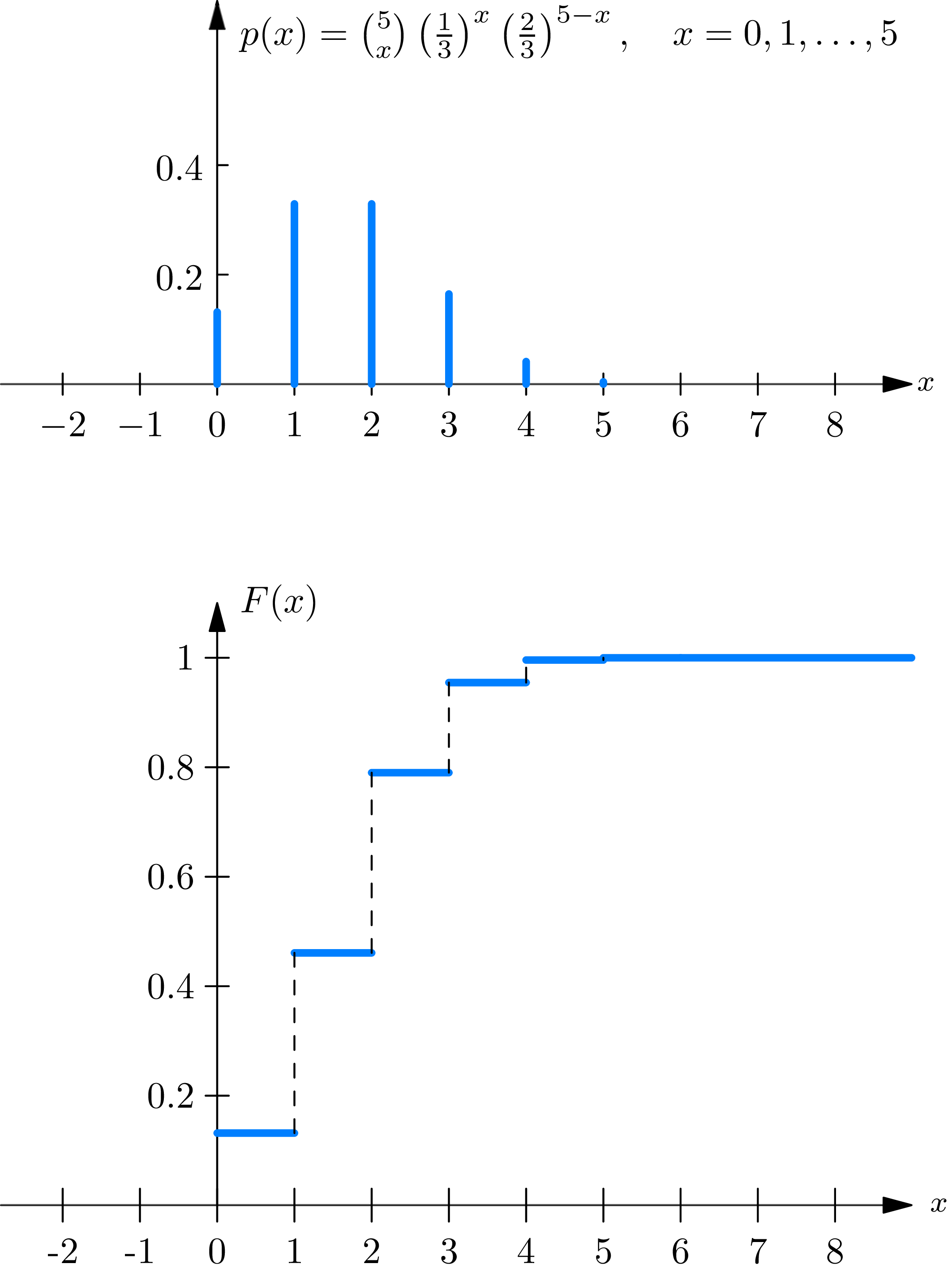
We may classify numerical valued random phenomena by classifying their distribution functions . To begin with, consider a random phenomenon whose probability function is specified by its probability mass function, so that its distribution function $F(\cdot )$ is given by (3.2) . The graph $y=F(x)$ then appears as it is shown in (Fig. 3A) ; it consists of a sequence of horizontal line segments, each one higher than its predecessor. The points at which one moves from one line to the next are called the jump points of the distribution function $F(\cdot )$ ; they occur at all points $x$ at which the probability mass function $p(x)$ is positive. We define a discrete distribution function as one that is given by a formula of the form of (3.2) , in terms of a probability mass function $p(\cdot )$ , or equivalently as one whose graph (Fig. 3A) consists only of jumps and level stretches. The term “discrete” connotes the fact that the numerical valued random phenomenon corresponding to a discrete distribution function could be assigned, as its sample description space, the set consisting of the (at most countably infinite number of) points at which the graph of the distribution function jumps.

Let us next consider a numerical valued random phenomenon whose probability function is specified by a probability density function, so that its distribution function $F(\cdot )$ is given by (3.3) . The graph $y=F(x)$ then appears (Fig. 3B) as an unbroken curve. The function $F(\cdot )$ is continuous. However, even more is true; the derivative exists at all points (except perhaps for a finite number of points) and is given by  

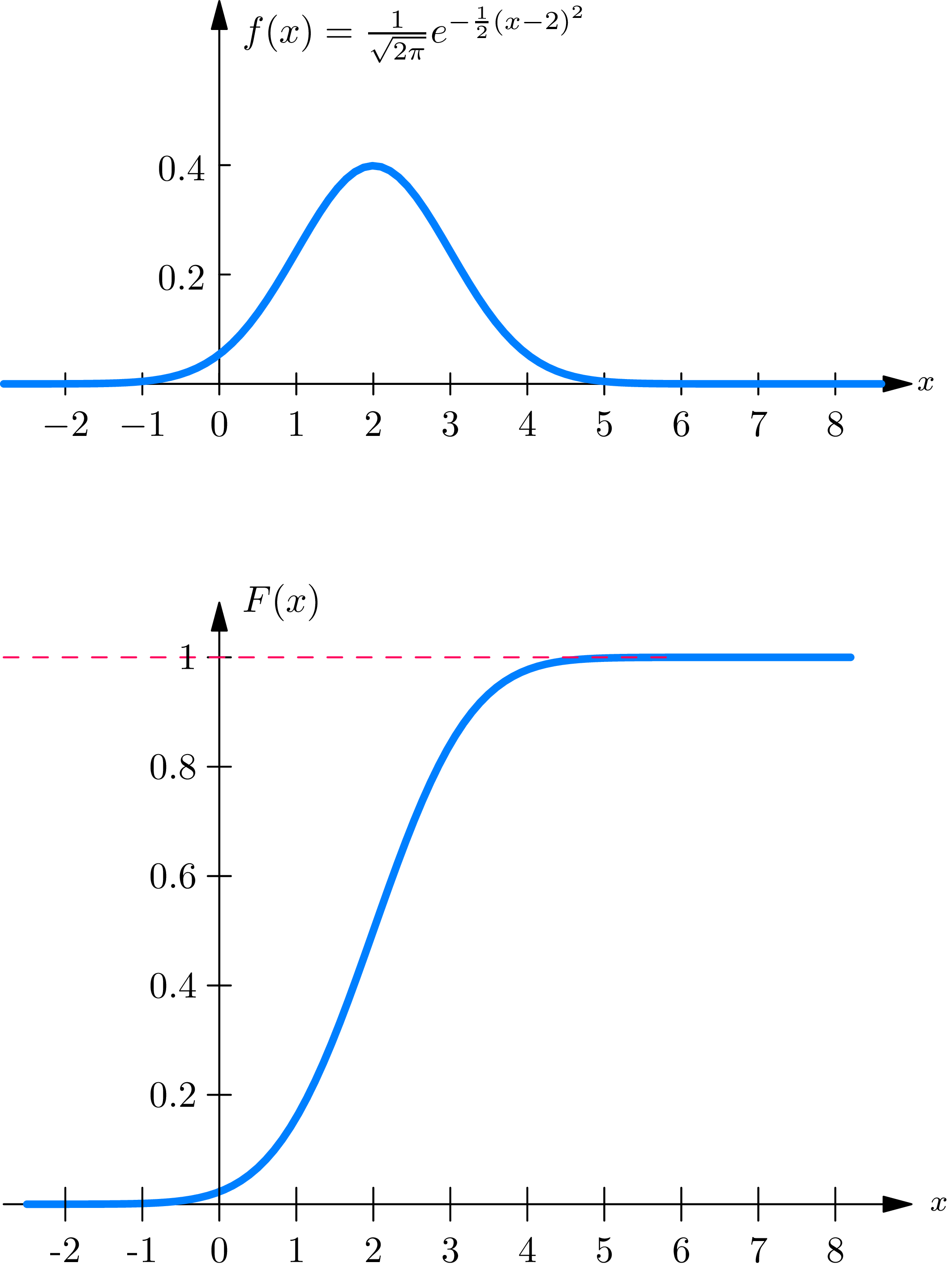
We define a continuous distribution function as one that is given by a formula of the form of (3.3) in terms of a probability density function.

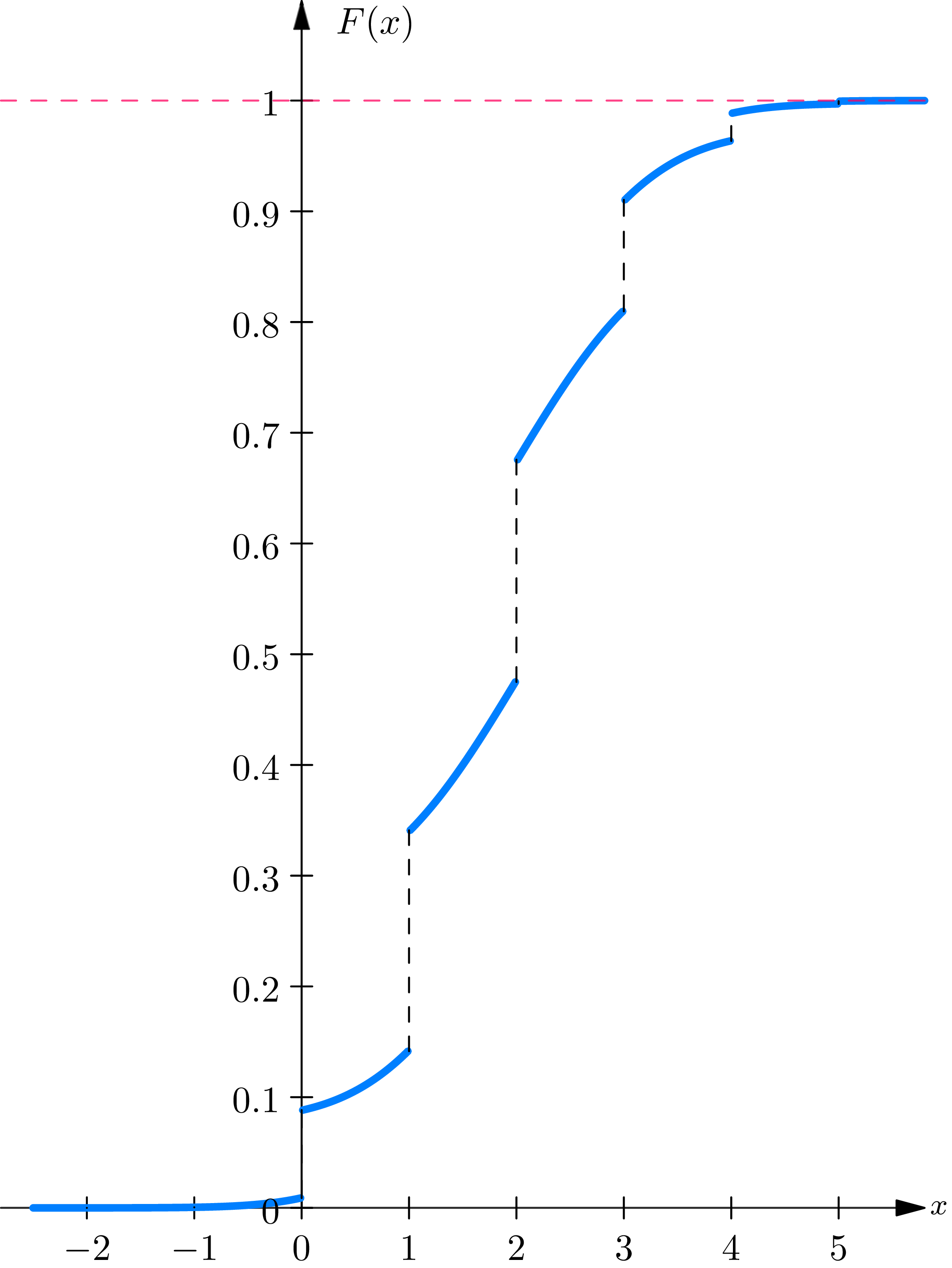
Most of the distribution functions arising in practice are either discrete or continuous. Nevertheless, it is important to realize that there are distribution functions, such as the one whose graph is shown in (Fig. 3C) , that are neither discrete nor continuous. Such distribution functions are called mixed . A distribution function $F(\cdot )$ is called mixed if it can be written as a linear combination of two distribution functions, denoted by $F^d(\cdot )$ and $F^c(\cdot )$ , which are discrete and continuous, respectively, in the following way: for any real number $x$ in which $c_1$ and $c_2$ are constants between 0 and 1, whose sum is one. The distribution function $F(\cdot )$ , graphed in Fig. 3C , is mixed, since $F(x)=$ $\frac{3}{5}{F}^d(x)+\frac{2}{5}{F}^c(x)$ , in which $F^d(\cdot )$ and $F^c(\cdot )$ are the distribution functions graphed in Fig. 3A and 3B, respectively.

Any numerical valued random phenomenon possesses a probability mass function $p(\cdot )$ defined as follows: for any real number $x$  

Thus $p(x)$ represents the probability that the random phenomenon will have an observed value equal to $x$ . In terms of the representation of the probability function as a distribution of a unit mass over the real line, $p(x)$ represents the mass (if any) concentrated at the point $x$ . It may be shown that $p(x)$ represents the size of the jump at $x$ in the graph of the distribution function $F(\cdot )$ of the numerical valued random phenomenon. Consequently, $p(x)=0$ for all $x$ if and only if $F(\cdot )$ is continuous.

We now introduce the following notation. Given a numerical valued random phenomenon, we write $X$ to denote the observed value of the random phenomenon. For any real numbers $a$ and $b$ we write $P[a\le X\le b]$ to mean the probability that an observed value $X$ of the numerical valued random phenomenon lies in the interval $a$ to $b$ . It is important to keep in mind that $P[a\le X\le b]$ represents an informal notation for $P[\{x:a\le x\le b\}]$ .

Some writers on probability theory call a number $X$ determined by the outcome of a random experiment (as is the observed value $X$ of a numerical valued random phenomenon) a random variable. In Chapter 7 we give a rigorous definition of the notion of random variable in terms of the notion of function, and show that the observed value $X$ of a numerical valued random phenomenon can be regarded as a random variable. For the present we have the following definition:

Given an observed value $X$ of a numerical valued random phenomenon with distribution function $F(\cdot )$ and probability mass function $p(\cdot )$ , we have the following formulas for any real numbers $a$ and $b$ (in which ): To prove (3.7) , define the events $A,B,C$ , and $D$ : $$A=\{X\le a\},B=\{X\le b\},C=\{X=a\},D=\{X=b\}.$$ Then (3.7) merely expresses the facts that (since $A\subset B,C\subset A,D\subset B$ )  

The use of (3.7) in solving probability problems posed in terms of distribution functions is illustrated in example 3A.

Example 3A . Suppose that the duration in minutes of long distance telephone calls made from a certain city is found to be a random phenomenon, with a probability function specified by the distribution function $F(\cdot )$ , given by in which the expression $[y]$ is defined for any real number $y\ge 0$ as the largest integer less than or equal to $y$ . What is the probability that the duration in minutes of a long distance telephone call is (i) more than six minutes, (ii) less than four minutes, (iii) equal to three minutes? What is the conditional probability that the duration in minutes of a long distance telephone call is (iv) less than nine minutes, given that it is more than five minutes, (v) more than five minutes, given that it is less than nine minutes?

 

Solution

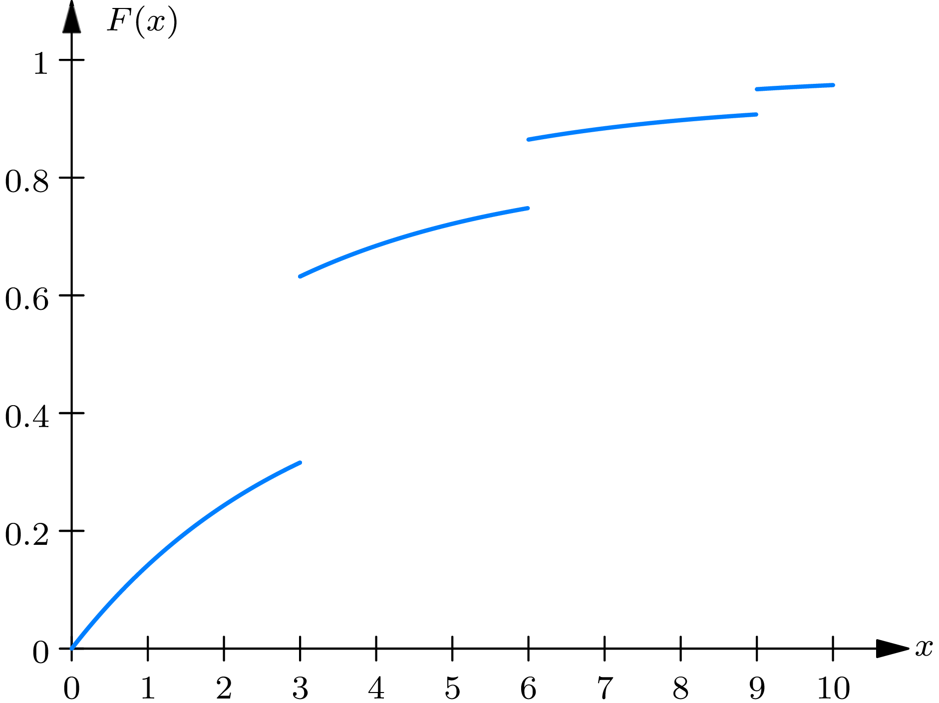
The distribution function given by (3.9) is neither continuous nor discrete but mixed. Its graph is given in (Fig. 3D) . For the sake of brevity, we write $X$ for the duration in minutes of a telephone call and as an abbreviation in mathematical symbols of the verbal statement “the probability that a telephone call has a duration strictly greater than six minutes”. The intuitive statement is identified in our model with , the value at the set of the probability function $P\left[{}^{\cdot }\right]$ corresponding to the distribution function $F(\cdot )$ given by (3.9) . Consequently, Next, the probability that the duration of a call will be less than four minutes (or, more concisely written, ) is equal to $F(4)-p(4)$ , in which $p(4)$ is the jump in the distribution function $F(\cdot )$ at $x=4$ . A glance at the graph of $F(\cdot )$ , drawn in (Fig. 3D) , reveals that the graph is unbroken at $x=4$ . Consequently, $p(4)=0$ , and  

 

观测到的通话时长$X$等于3的概率$P[X=3]$由下式给出其中$p(3)$是$F(\cdot )$在$x=3$处图形的跳跃。该示例第(iv)和(v)部分的解可以类似地得到： 

在第2节中，我们给出了一个函数必须满足的条件，才能成为概率密度函数或概率质量函数。自然会产生一个问题：一个函数必须满足什么条件才能成为分布函数。在概率论的高级研究中表明，一个函数$F(\cdot )$要成为分布函数必须具备以下性质：(i) $F(\cdot )$必须是非递减的，即对于任意实数$a$和$b$， 

(ii) $F(x)$当$x$趋于正无穷或负无穷时的极限必须存在，并由下式给出 

(iii) 在任意点$x$处，右极限$\underset{b\to x+}{lim}F(b)$（定义为当$b$通过大于$x$的值趋于$x$时$F(b)$的极限）必须等于$F(x)$， 因此在任意点$x$处，当从右侧趋近$x$时，$F(x)$的图形是连续的；(iv) 在任意点$x$处，左极限，记作$F(x-)$或$limF(a)$（定义为当$a$通过小于$x$的值$a\to x-$趋于$x$时$F(a)$的极限），必须等于$F(x)-p(x)$；用符号表示为， 其中我们定义$p(x)$为随机现象的观测值等于$x$的概率。注意$p(x)$表示$F(x)$在$x$处图形跳跃的大小。

由这些事实可知，一个典型分布函数$F(\cdot )$的图形$y=F(x)$以直线$y=0$和$y=1$为其渐近线。该图形是非递减的。然而，它不需要在每一点都增加，而可以在某些区间上保持水平（平坦）。该图形不需要在所有点都连续[即$F(\cdot )$不需要连续]，但至多有可数无穷多个点处图形有间断；在这些点处它向上跳跃，并具有右极限和左极限，满足(3.12)和(3.13)。

上述数值随机现象分布函数的数学性质完全刻画了这类函数。可以证明，对于任何具有所列前三个性质的函数，存在唯一的集函数$P[\cdot ]$，定义在实直线的Borel集上，满足第1节的公理$1-3$以及条件：对于任意有限实数$a$和$b$，其中$a\le b$， 由这一事实可知，要指定概率函数，只需指定分布函数即可。

分布函数连续这一事实并不意味着它可以用概率密度函数通过诸如(3.3)这样的公式来表示。如果可以这样表示，则称其为绝对连续。还存在另一种连续分布函数，称为奇异连续，其导数几乎处处为零。这是一个较难想象的概念，例子只能通过相当复杂的分析运算来构造。从实际角度来看，我们可以认为奇异分布函数不存在，因为这类函数的例子在实践中即使有也极少遇到。可以证明，任何分布函数都可以表示为如下形式 其中$F^d(\cdot ),F^{ac}(\cdot )$和$F^{sc}(\cdot )$分别是离散的、绝对连续的和奇异连续的，而$c_1,c_2$和$c_3$是介于0和1之间（含）的常数，其和为1。如果假设对于实践中遇到的任何分布函数，系数$c_3$为零，那么要研究分布函数的性质，只需研究那些离散的或连续的就足够了。

理论练习

练习