To describe completely a numerical-valued random phenomenon, one needs only to state its probability function. The probability function \(P\left[{\cdot}\right]\) is a function of sets and for this reason is somewhat unwieldy to treat analytically. It would be preferable if there were a function of points (that is, a function of real numbers \(x\) ), which would suffice to determine completely the probability function. In the case of a probability function, specified by a probability density function or by a probability mass function, the density and mass functions provide a point function that determines the probability function. Now it may be shown that for any numerical valued random phenomenon whatsoever there exists a point function, called the distribution function, which suffices to determine the probability function in the sense that the probability function may be reconstructed from the distribution function. The distribution function (often referred to as the cumulative distribution function or CDF ) thus provides a point function that contains all the information necessary to describe the probability properties of the random phenomenon. Consequently, to study the general properties of numerical valued random phenomena without restricting ourselves to those whose probability functions are specified by either a probability density function or by a probability mass function, it suffices to study the general properties of distribution functions.
The (cumulative) distribution function \(F(\cdot)\) of a numerical valued random phenomenon is defined as having as its value, at any real number \(x\) , the probability that an observed value of the random phenomenon will be less than or equal to the number \(x\) . In symbols, for any real number \(x\) , \[F(x)=P\left[\left\{\text {real numbers } x^{\prime}: x^{\prime} \leq x\right\}\right]. \tag{3.1}\]
Before discussing the general properties of distribution functions, let us consider the distribution functions of numerical valued random phenomena, whose probability functions are specified by either a probability mass function or a probability density function. If the probability function is specified by a probability mass function \(p(\cdot)\) , then the corresponding distribution function \(F(\cdot)\) for any real number \(x\) is given by \[F(x)=\sum_{\substack{\text { points } x^{\prime} \leq x \\ \text { such that } p\left(x^{\prime}\right)>0}} p\left(x^{\prime}\right). \tag{3.2}\]
Equation (3.2) follows immediately from (3.1) and (2.7) . If the probability function is specified by a probability density function \(f(\cdot)\) , then the corresponding distribution function \(F(\cdot)\) for any real number \(x\) is given by \[F(x)=\int_{-\infty}^{x} f\left(x^{\prime}\right) d x^{\prime}. \tag{3.3}\]
Equation (3.3) follows immediately from (3.1) and (2.1) .
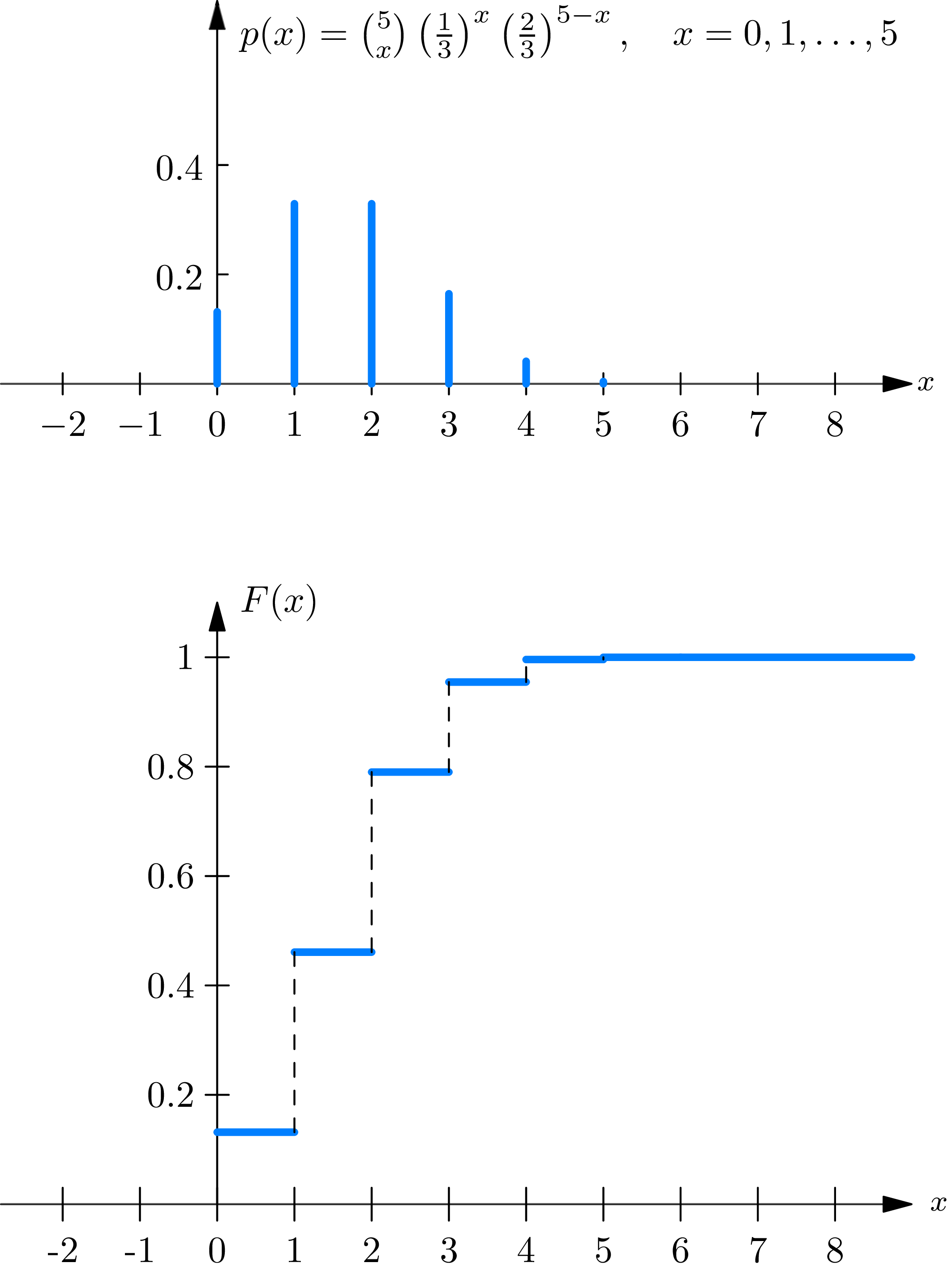
We may classify numerical valued random phenomena by classifying their distribution functions . To begin with, consider a random phenomenon whose probability function is specified by its probability mass function, so that its distribution function \(F(\cdot)\) is given by (3.2) . The graph \(y=F(x)\) then appears as it is shown in (Fig. 3A) ; it consists of a sequence of horizontal line segments, each one higher than its predecessor. The points at which one moves from one line to the next are called the jump points of the distribution function \(F(\cdot)\) ; they occur at all points \(x\) at which the probability mass function \(p(x)\) is positive. We define a discrete distribution function as one that is given by a formula of the form of (3.2) , in terms of a probability mass function \(p(\cdot)\) , or equivalently as one whose graph (Fig. 3A) consists only of jumps and level stretches. The term “discrete” connotes the fact that the numerical valued random phenomenon corresponding to a discrete distribution function could be assigned, as its sample description space, the set consisting of the (at most countably infinite number of) points at which the graph of the distribution function jumps.

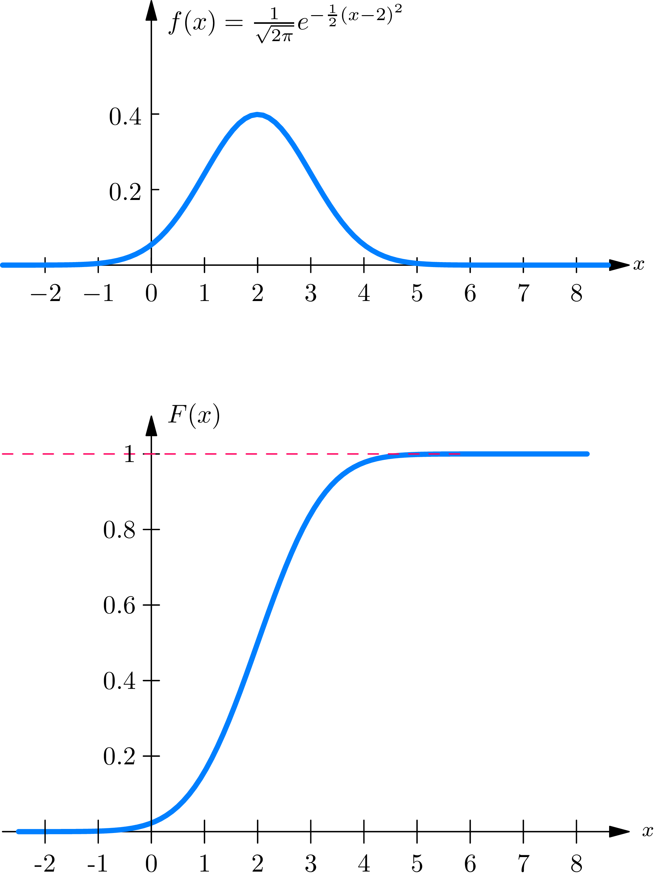
Let us next consider a numerical valued random phenomenon whose probability function is specified by a probability density function, so that its distribution function \(F(\cdot)\) is given by (3.3) . The graph \(y=F(x)\) then appears (Fig. 3B) as an unbroken curve. The function \(F(\cdot)\) is continuous. However, even more is true; the derivative \(F^{\prime}(x)\) exists at all points (except perhaps for a finite number of points) and is given by \[F^{\prime}(x)=\frac{d}{d x} F(x)=f(x). \tag{3.4}\]

We define a continuous distribution function as one that is given by a formula of the form of (3.3) in terms of a probability density function.
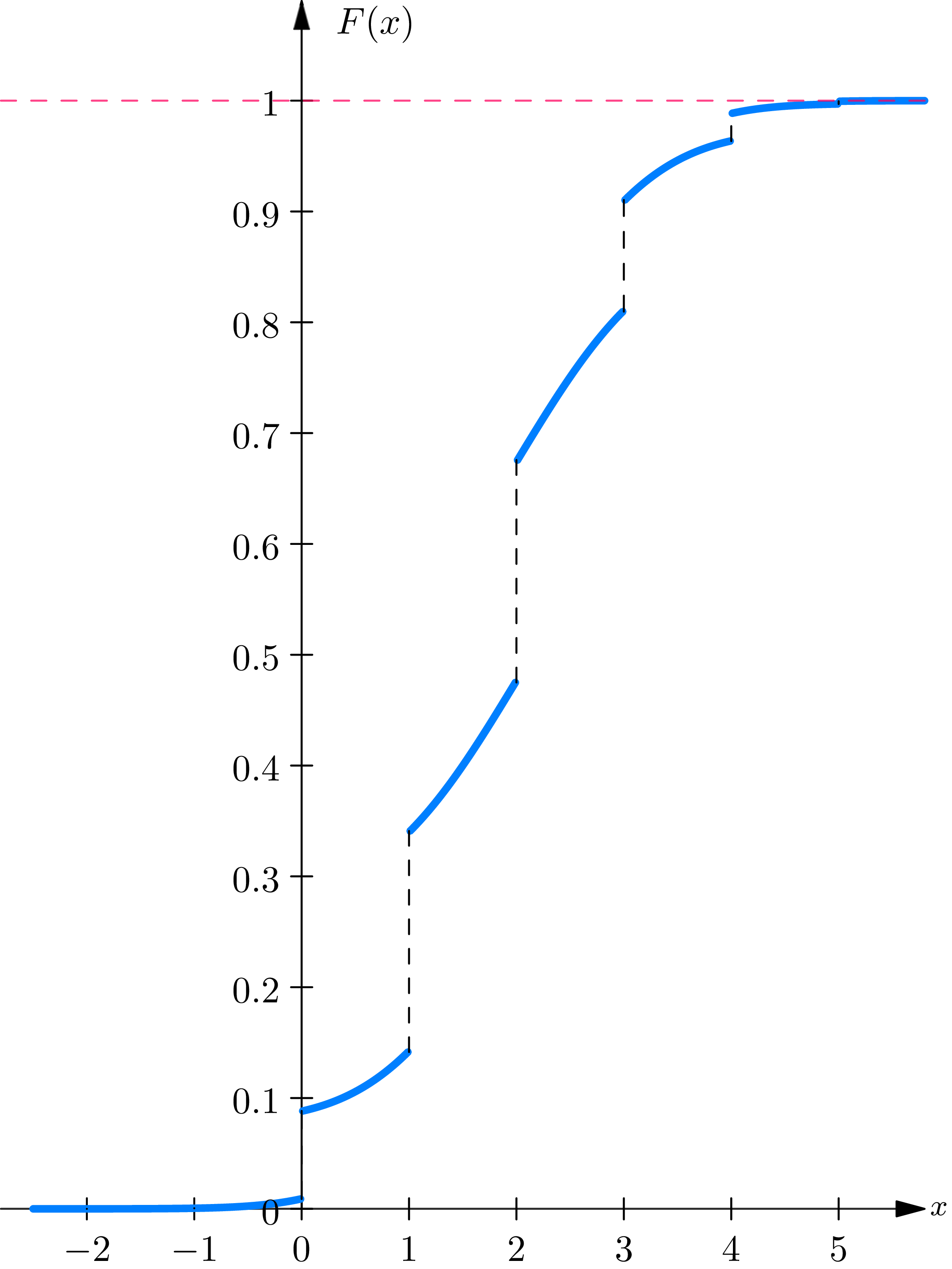
Most of the distribution functions arising in practice are either discrete or continuous. Nevertheless, it is important to realize that there are distribution functions, such as the one whose graph is shown in (Fig. 3C) , that are neither discrete nor continuous. Such distribution functions are called mixed . A distribution function \(F(\cdot)\) is called mixed if it can be written as a linear combination of two distribution functions, denoted by \(F^{d}(\cdot)\) and \(F^{c}(\cdot)\) , which are discrete and continuous, respectively, in the following way: for any real number \(x\) \[F(x)=c_{1} F^{d}(x)+c_{2} F^{c}(x), \tag{3.5}\] in which \(c_{1}\) and \(c_{2}\) are constants between 0 and 1, whose sum is one. The distribution function \(F(\cdot)\) , graphed in Fig. 3C , is mixed, since \(F(x)=\) \(\frac{3}{5} F^{d}(x)+\frac{2}{5} F^{c}(x)\) , in which \(F^{d}(\cdot)\) and \(F^{c}(\cdot)\) are the distribution functions graphed in Fig. 3A and 3B, respectively.

Any numerical valued random phenomenon possesses a probability mass function \(p(\cdot)\) defined as follows: for any real number \(x\) \[p(x)=P\left[\left\{\text { real numbers } x^{\prime}: x^{\prime}=x\right\}\right]=P[\{x\}]. \tag{3.6}\]
Thus \(p(x)\) represents the probability that the random phenomenon will have an observed value equal to \(x\) . In terms of the representation of the probability function as a distribution of a unit mass over the real line, \(p(x)\) represents the mass (if any) concentrated at the point \(x\) . It may be shown that \(p(x)\) represents the size of the jump at \(x\) in the graph of the distribution function \(F(\cdot)\) of the numerical valued random phenomenon. Consequently, \(p(x)=0\) for all \(x\) if and only if \(F(\cdot)\) is continuous.
We now introduce the following notation. Given a numerical valued random phenomenon, we write \(X\) to denote the observed value of the random phenomenon. For any real numbers \(a\) and \(b\) we write \(P[a \leq X \leq b]\) to mean the probability that an observed value \(X\) of the numerical valued random phenomenon lies in the interval \(a\) to \(b\) . It is important to keep in mind that \(P[a \leq X \leq b]\) represents an informal notation for \(P[\{x: a \leq x \leq b\}]\) .
Some writers on probability theory call a number \(X\) determined by the outcome of a random experiment (as is the observed value \(X\) of a numerical valued random phenomenon) a random variable. In Chapter 7 we give a rigorous definition of the notion of random variable in terms of the notion of function, and show that the observed value \(X\) of a numerical valued random phenomenon can be regarded as a random variable. For the present we have the following definition:
\(A\) quantity \(X\) is said to be a random variable (or, equivalently, \(X\) is said to be an observed value of a numerical valued random phenomenon) if for every real number \(x\) there exists a probability (which we denote by \(P[X \leq x]\) ) that \(X\) is less than or equal to \(x\) .
Given an observed value \(X\) of a numerical valued random phenomenon with distribution function \(F(\cdot)\) and probability mass function \(p(\cdot)\) , we have the following formulas for any real numbers \(a\) and \(b\) (in which \(a<b\) ): \begin{align} & P[a<X \leq b]=P[\{x: a<x \leq b\}]=F(b)-F(a) \\ & P[a \leq X \leq b]=P[\{x: a \leq x \leq b\}]=F(b)-F(a)+p(a) \\ & P[a \leq X<b]=P[\{x: a \leq x<b\}]=F(b)-F(a)+p(a)-p(b) \tag{3.7} \\ & P[a<X<b]=P[\{x: a<x<b\}]=F(b)-F(a)-p(b) \end{align} To prove (3.7) , define the events \(A, B, C\) , and \(D\) : \[A=\{X \leq a\}, \quad B=\{X \leq b\}, \quad C=\{X=a\}, \quad D=\{X=b\}.\] Then (3.7) merely expresses the facts that (since \(A \subset B, C \subset A, D \subset B\) ) \begin{align} P\left[B A^{c}\right] & =P[B]-P[A] \\ P\left[B A^{c} \cup C\right] & =P[B]-P[A]+P[C] \\ P\left[B A^{c} D^{c} \cup C\right] & =P[B]-P[A]+P[C]-P[D] \tag{3.8} \\ P\left[B A^{c} D^{c}\right] & =P[B]-P[A]-P[D]. \end{align}
The use of (3.7) in solving probability problems posed in terms of distribution functions is illustrated in example 3A.
Example 3A . Suppose that the duration in minutes of long distance telephone calls made from a certain city is found to be a random phenomenon, with a probability function specified by the distribution function \(F(\cdot)\) , given by \begin{align} F(x) = \begin{cases} 0, & \text{for } x < 0 \\[2mm] 1 - \frac{1}{2} e^{-\frac{x}{3}} - \frac{1}{2} e^{-\left[\frac{x}{3}\right]}, & \text{for } x \geq 0, \tag{3.9} \end{cases} \end{align} in which the expression \([y]\) is defined for any real number \(y \geq 0\) as the largest integer less than or equal to \(y\) . What is the probability that the duration in minutes of a long distance telephone call is (i) more than six minutes, (ii) less than four minutes, (iii) equal to three minutes? What is the conditional probability that the duration in minutes of a long distance telephone call is (iv) less than nine minutes, given that it is more than five minutes, (v) more than five minutes, given that it is less than nine minutes?
Solution
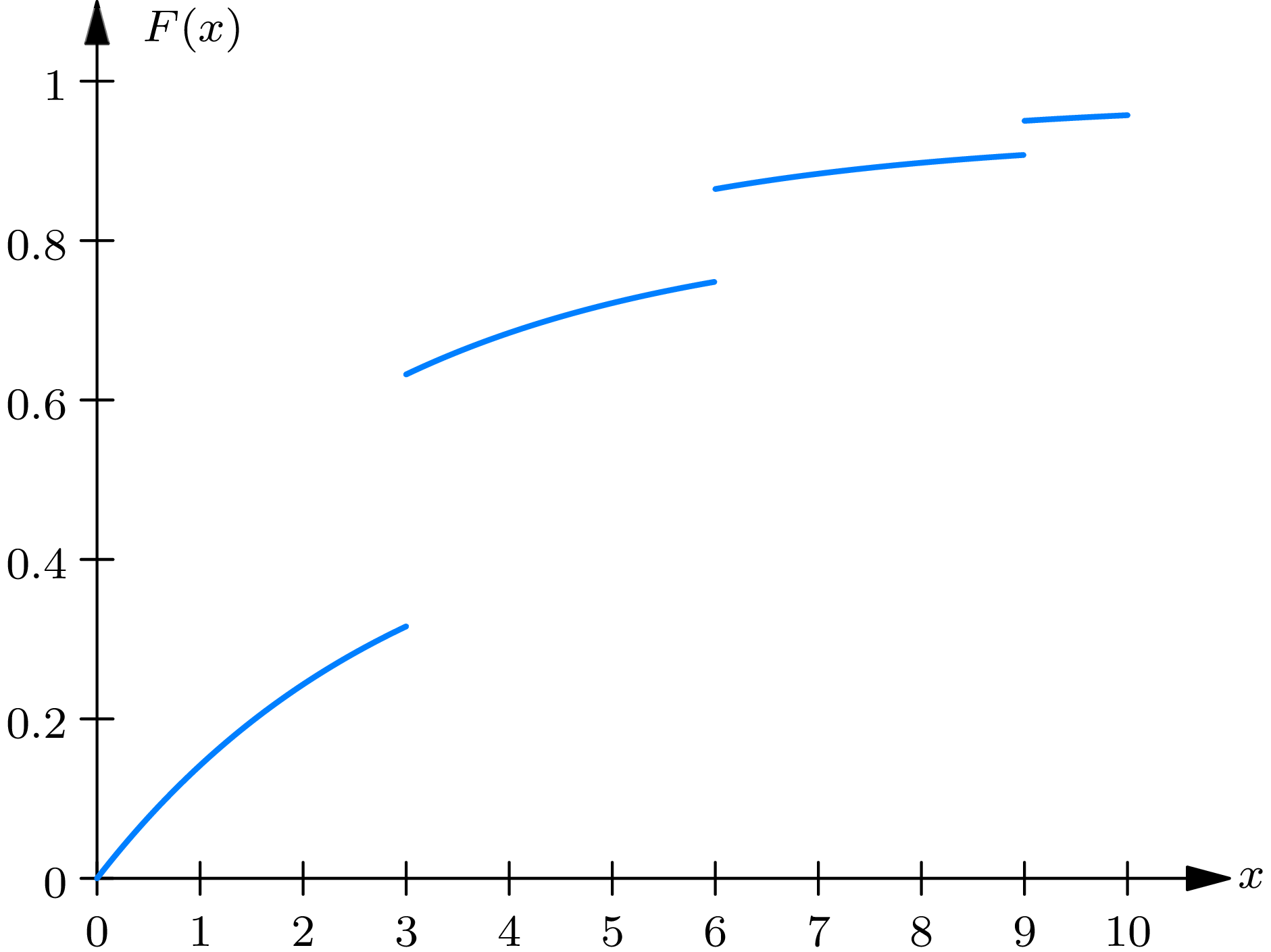
The distribution function given by (3.9) is neither continuous nor discrete but mixed. Its graph is given in (Fig. 3D) . For the sake of brevity, we write \(X\) for the duration in minutes of a telephone call and \(P[X>6]\) as an abbreviation in mathematical symbols of the verbal statement “the probability that a telephone call has a duration strictly greater than six minutes”. The intuitive statement \(P[X>6]\) is identified in our model with \(P\left[\left\{x^{\prime}: x^{\prime}>6\right\}\right]\) , the value at the set \(\left\{x^{\prime}: x^{\prime}>6\right\}\) of the probability function \(P\left[^{\cdot}\right]\) corresponding to the distribution function \(F(\cdot)\) given by (3.9) . Consequently, \[P[X>6]=1-F(6)=\frac{1}{2} e^{-2}+\frac{1}{2} e^{-[2]}=e^{-2}=0.135.\] Next, the probability that the duration of a call will be less than four minutes (or, more concisely written, \(P[X<4]\) ) is equal to \(F(4)-p(4)\) , in which \(p(4)\) is the jump in the distribution function \(F(\cdot)\) at \(x=4\) . A glance at the graph of \(F(\cdot)\) , drawn in (Fig. 3D) , reveals that the graph is unbroken at \(x=4\) . Consequently, \(p(4)=0\) , and \[P[X<4]=1-\frac{1}{2} e^{-(4 / 3)}-\frac{1}{2} e^{-[4 / 3]}=1-\frac{1}{2} e^{-(4 / 3)}-\frac{1}{2} e^{-1}=0.684.\]

The probability \(P[X=3]\) that an observed value \(X\) of the duration of a call is equal to 3 is given by \begin{align} P[X=3] & =p(3)=\left(1-\frac{1}{2} e^{-(3 / 3)}-\frac{1}{2} e^{-[3 / 3]}\right)-\left(1-\frac{1}{2} e^{-(3 / 3)}-\frac{1}{2} e^{-[2 / 3]}\right) \\ & =\frac{1}{2}\left(1-e^{-1}\right)=0.316, \end{align} in which \(p(3)\) is the jump in the graph of \(F(\cdot)\) at \(x=3\) . Solutions to parts (iv) and (v) of the example may be obtained similarly: \begin{align} P[X<9 \mid X>5] & =\frac{P[5<X<9]}{P[X>5]}=\frac{F(9)-p(9)-F(5)}{1-F(5)} \\[2mm] & =\frac{\frac{1}{2}\left(e^{-(5 / 3)}+e^{-1}-e^{-3}-e^{-2}\right)}{\frac{1}{2}\left(e^{-(5 / 3)}+e^{-1}\right)} \\[2mm] & =\frac{0.187}{0.279}=0.670, \\[2mm] P[X>5 \mid X<9] & =\frac{P[5<X<9]}{P[X<9]}=\frac{F(9)-p(9)-F(5)}{F(9)-p(9)} \\[2mm] & =\frac{\frac{1}{2}\left(e^{-(5 / 3)}+e^{-1}-e^{-3}-e^{-2}\right)}{\frac{1}{2}\left(2-e^{-3}-e^{-2}\right)} \\[2mm] & =\frac{0.187}{0.908}=0.206. \end{align}
In section 2 we gave the conditions a function must satisfy in order to be a probability density function or a probability mass function. The question naturally arises as to the conditions a function must satisfy in order to be a distribution function. In advanced studies of probability theory it is shown that the properties a function \(F(\cdot)\) must have in order to be a distribution function are the following: (i) \(F(\cdot)\) must be non-decreasing in the sense that for any real numbers \(a\) and \(b\) \[F(a) \leq F(b) \quad \text { if } a<b; \tag{3.10}\]
(ii) the limits of \(F(x)\) , as \(x\) tends to either plus or minus infinity, must exist and be given by \[\lim _{x \rightarrow-\infty} F(x)=0, \quad \lim _{x \rightarrow \infty} F(x)=1; \tag{3.11}\]
(iii) at any point \(x\) the limit from the right \(\lim_{b \rightarrow x+} F(b)\) , which is defined as the limit of \(F(b)\) , as \(b\) tends to \(x\) through values greater than \(x\) , must be equal to \(F(x)\) , \[\lim _{b \rightarrow x+} F(b)=F(x) \tag{3.12}\] so that at any point \(x\) the graph of \(F(x)\) is unbroken as one approaches \(x\) from the right; (iv) at any point \(x\) , the limit from the left, written \(F(x-)\) or \(\lim F(a)\) , which is defined as the limit of \(F(a)\) as \(a\) tends to \(x\) through \(a \rightarrow x-\) values less than \(x\) , must be equal to \(F(x)-p(x)\) ; in symbols, \[F(x-)=\lim _{a \rightarrow x-} F(a)=F(x)-p(x), \tag{3.13}\] where we define \(p(x)\) as the probability that the observed value of the random phenomenon is equal to \(x\) . Note that \(p(x)\) represents the size of the jump in the graph of \(F(x)\) at \(x\) .
From these facts it follows that the graph \(y=F(x)\) of a typical distribution function \(F(\cdot)\) has as its asymptotes the lines \(y=0\) and \(y=1\) . The graph is non-decreasing. However, it need not increase at every point but rather may be level (horizontal) over certain intervals. The graph need not be unbroken [that is, \(F(\cdot)\) need not be continuous] at all points, but there is at most a countable infinity of points at which the graph has a break; at these points it jumps upward and possesses limits from the right and the left, satisfying (3.12) and (3.13) .
The foregoing mathematical properties of the distribution function of a numerical valued random phenomenon serve to characterize completely such functions. It may be shown that for any function possessing the first three properties listed there is a unique set function \(P[\cdot]\) , defined on the Borel sets of the real line, satisfying axioms \(1-3\) of section 1 and the condition that for any finite real numbers \(a\) and \(b\) , at which \(a \leq b\) , \[P[\{\text { real numbers } x: \ a<x \leq b\}]=F(b)-F(a). \tag{3.14}\] From this fact it follows that to specify the probability function it suffices to specify the distribution function.
The fact that a distribution function is continuous does not imply that it may be represented in terms of a probability density function by a formula such as (3.3) . If this is the case, it is said to be absolutely continuous . There also exists another kind of continuous distribution function, called singular continuous , whose derivative vanishes at almost all points. This is a somewhat difficult notion to picture, and examples have been constructed only by means of fairly involved analytic operations. From a practical point of view, one may act as if singular distribution functions do not exist, since examples of these functions are rarely, if ever, encountered in practice. It may be shown that any distribution function may be represented in the form \[F(x)=c_{1} F^{d}(x)+c_{2} F^{a c}(x)+c_{3} F^{s c}(x), \tag{3.15}\] in which \(F^{d}(\cdot), F^{a c}(\cdot)\) , and \(F^{s c}(\cdot)\) , respectively, are discrete, absolutely continuous, and singular continuous, and \(c_{1}, c_{2}\) , and \(c_{3}\) are constants between 0 and 1, inclusive, the sum of which is 1. If it is assumed that the coefficient \(c_{3}\) vanishes for any distribution function encountered in practice, it follows that in order to study the properties of a distribution function it suffices to study those that are discrete or continuous.
Theoretical Exercises
3.1 . Show that the probability mass function \(p(\cdot)\) of a numerical valued random phenomenon can be positive at no more than a countable infinity of points.
Hint : For \(n=2,3, \ldots\) , define \(E_{n}\) as the set of points \(x\) at which \(p(x)>(1 / n)\) . The size of \(E_{n}\) is less than \(n\) , for if it were greater than \(n\) it would follow that \(P\left[E_{n}\right]>1\) . Thus each of the sets \(E_{n}\) is of finite size. Now the set \(E\) of points \(x\) at which \(p(x)>0\) is equal to the union \(E_{2} \cup\) \(E_{3} \cup \ldots \cup E_{n} \cup \ldots\) , since \(p(x)>0\) if and only if; for some integer \(n\) , \(p(x)>(1 / n)\) . The set \(E\) , being a union of a countable number of sets of finite size, is therefore proved to have at most a countable infinity of members.
Exercises
3.1 - 3.7 . For \(k=1,2, \ldots, 7\) , exercise \(3 . k\) is to sketch the distribution function corresponding to each probability density function or probability mass function given in exercise \(2.k\) .
3.8 . In the game of “odd man out” (described in section 3 of Chapter 3) the number of trials required to conclude the game, if there are 5 players, is a numerical valued random phenomenon, with a probability function specified by the distribution function \(F(\cdot)\) , given by \begin{align} F(x) = \begin{cases} 0, & \text{for } x < 1 \\[2mm] 1 - \left(\frac{11}{16}\right)^{[x]}, & \text{for } x \geq 1, \end{cases} \end{align} in which \([x]\) denotes the largest integer less than or equal to \(x\) .
(i) Sketch the distribution function.
(ii) Is the distribution function discrete? If so, give a formula for its probability mass function.
(iii) What is the probability that the number of trials required to conclude the game will be (a) more than \(3,(b)\) less than \(3,(c)\) equal to \(3,(d)\) between 2 and 5, inclusive.
(iv) What is the conditional probability that the number of trials required to conclude the game will be (a) more than 5, given that it is more than 3 trials, \((b)\) more than 3, given that it is more than 5 trials?
3.9 . Suppose that the amount of money (in dollars) that a person in a certain social group has saved is found to be a random phenomenon, with a probability function specified by the distribution function \(F(\cdot)\) , given by
\begin{align} F(x) = \begin{cases} \frac{1}{2} e^{-(x/50)^{2}}, & \text{for } x \leq 0 \\[2mm] 1 - \frac{1}{2} e^{-(x/50)^{2}}, & \text{for } x \geq 0. \end{cases} \end{align}
Note that a negative amount of savings represents a debt.
(i) Sketch the distribution function.
(ii) Is the distribution function continuous? If so, give a formula for its probability density function.
(iii) What is the probability that the amount of savings possessed by a person in the group will be (a) more than 50 dollars, \((b)\) less than -50 dollars, \((c)\) between -50 dollars and 50 dollars, \((d)\) equal to 50 dollars? (iv) What is the conditional probability that the amount of savings possessed by a person in the group will be (a) less than 100 dollars, given that it is more than 50 dollars, (b) more than \(50\) dollars, given that it is less than 100 dollars?
Answer
(ii) \(f(x)=\frac{|x|}{2500} e^{-(x / 50)^{2}}\) ; (iii) (a), (b) 0.184, (c) 0.632, (d) 0; (iv) (a) \(1-e^{-1}\) , (b) \(\left(e^{-1}-e^{-4}\right) /\left(2-e^{-4}\right)\) .
3.10 . Suppose that the duration in minutes of long-distance telephone calls made from a certain city is found to be a random phenomenon, with a probability function specified by the distribution function \(F(\cdot)\) , given by \begin{align} F(x) = \begin{cases} 0, & \text{for } x \leq 0 \\[2mm] 1 - \frac{2}{3} e^{-\frac{x}{3}} - \frac{1}{3} e^{-\left[\frac{x}{3}\right]}, & \text{for } x > 0. \end{cases} \end{align}
(i) Sketch the distribution function.
(ii) Is the distribution function continuous? Discrete? Neither?
(iii) What is the probability that the duration in minutes of a long-distance telephone call will be (a) more than 6 minutes, \((b)\) less than 4 minutes, (c) equal to 3 minutes, \((d)\) between 4 and 7 minutes?
(iv) What is the conditional probability that the duration of a long distance telephone call will be (a) less than 9 minutes, given that it has lasted more than 5 minutes, \((b)\) less than 9 minutes, given that it has lasted more than 15 minutes?
3.11 . Suppose that the time in minutes that a man has to wait at a certain subway station for a train is found to be a random phenomenon, with a probability function specified by the distribution function \(F(\cdot)\) , given by \begin{align} F(x) = \begin{cases} 0, & \text{for } x \leq 0 \\[2mm] \frac{1}{2} x, & \text{for } 0 \leq x \leq 1 \\[2mm] \frac{1}{2}, & \text{for } 1 \leq x \leq 2 \\[2mm] \frac{1}{4} x, & \text{for } 2 \leq x \leq 4 \\[2mm] 1, & \text{for } x \geq 4. \end{cases} \end{align}
(i) Sketch the distribution function.
(ii) Is the distribution function continuous? If so, give a formula for its probability density function.
(iii) What is the probability that the time the man will have to wait for a train will be (a) more than 3 minutes, \((b)\) less than 3 minutes, (c) between 1 and 3 minutes?
(iv) What is the conditional probability that the time the man will have to wait for a train will be (a) more than 3 minutes, given that it is more than 1 minute, (b) less than 3 minutes, given that it is more than 1 minute?
Answer
(ii) \(f(x)=\frac{1}{2}\) for \(0<x<1\) ; = \(\frac{1}{4}\) for \(2<x<4\) ; \(=0\) otherwise; (iii) (a) \(\frac{1}{4}\) , (b) \(\frac{3}{4}\) , (c) \(\frac{1}{4}\) ; (iv) (a) \(\frac{1}{2},(b) \frac{1}{2}\) .
3.12 . Consider a numerical valued random phenomenon with distribution function \begin{align} F(x) = \begin{cases} 0, & \text{for } x \leq 0 \\[2mm] \left(\frac{1}{4}\right) x, & \text{for } 0 < x < 1 \\[2mm] \frac{1}{3}, & \text{for } 1 \leq x \leq 2 \\[2mm] \left(\frac{1}{6}\right) x, & \text{for } 2 < x \leq 3 \\[2mm] \frac{1}{2}, & \text{for } 3 < x \leq 4 \\[2mm] \left(\frac{1}{8}\right) x, & \text{for } 4 < x \leq 8 \\[2mm] 1, & \text{for } 8 < x. \end{cases} \end{align}
What is the conditional probability that the observed value of the random phenomenon will be between 2 and 5, given that it is between 1 and 6, inclusive.