In order to determine the ability of the beam to withstand safely the applied loads, it is necessary to know the distribution of the internal forces in the beam. The complete solution of this problem is given in books on the Theory of Elasticity and Strength of Materials, but the necessary first steps in the solution involve only the principles of statics.
To find the internal forces in a beam at a particular section, one can imagine that the beam is cut at that section, and a free-body diagram of one portion of the beam can be drawn. Consider, for example, the simply supported beam with a single concentrated load, as shown in Fig. 1a, and suppose that we wish to know the internal forces in the beam at a section a distance \(x\) from the left reaction.
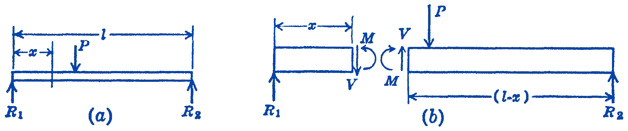
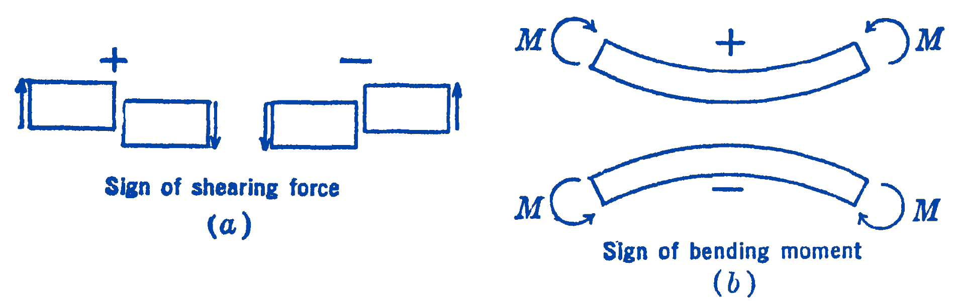
In Fig. 1b the beam is shown cut at the section \(x\) into two free-body diagrams. The actual forces acting on the cut cross section can be represented as in this example, but for our present purpose all that we require is the resultant of all of the forces normal to the beam axis, which we shall call the shearing force \(V\) in the beam, and the moment of the couple formed by the compression forces on the top portion of the beam and the tension forces on the bottom portion of the beam, which we shall call the bending moment \(M\) in the beam. Our present purpose is the determination of this shearing force and this bending moment for each section of the beam. From the complete free-body diagram of the beam shown in Fig. 1a, the two reaction forces \(R_{1}\) and \(R_{2}\) can be found. Thus, the free-body diagram of either end of the beam in Fig. 1b will contain only the two unknowns \(V\) and \(M\), which can therefore be found directly from the equations of statics. To decide on a sign convention for \(V\) and \(M\), we note that the shearing force on the left section is directed downward, while the shearing force on the right section, being the equal and opposite reaction of the other force, is directed upward. In order, however, to have one sign for the shearing force at one point in the beam, the convention is adopted that, if the shear in a beam is in such a direction that the right portion of the beam would tend to move downward with respect to the left portion, the shearing force at that point is positive. For a similar reason, a bending moment which tends to bend the beam concave upward is called a positive bending moment. These conventions are illustrated in Fig. 2.
The way in which the shearing force and the bending moment vary along a beam is usually shown by drawing a diagram beneath the beam as in the following examples. It should be noted that the same shearing force and bending moments will be computed for both portions of the beam. One usually selects as a free-body diagram the portion of the beam which involves the smaller number of forces.
The bending moment diagram can be drawn directly by a graphical method from the known beam loadings. This method follows directly from the discussion of the graphical determination of a bending moment by means of a funicular polygon. Since by definition the bending moment at a point in a beam is the sum of all of the moments of all of the forces on the beam to one side of the point, it follows that the funicular polygon as drawn in this problem, is the bending moment diagram for the beam.
Example 1. Draw the shearing force and bending moment diagrams for the simply supported beam with two concentrated loads shown in Fig. 3.
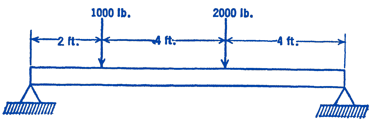
Solution. From a free-body diagram (Fig. 4) of the whole beam, the reaction forces can be found:
\(\sum M_{A}=0=-(2)(1000)-(6)(2000)+(10)\left(R_{2}\right) ; \quad R_{2}=1400\ \mathrm{lb}\)
\(\sum F_y=0=R_{1}+1400-1000-2000 ; \quad R_{1}=1600\ \mathrm{lb}\)
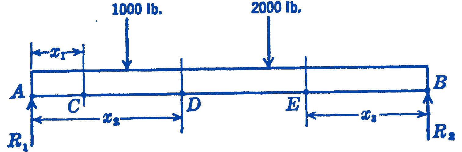
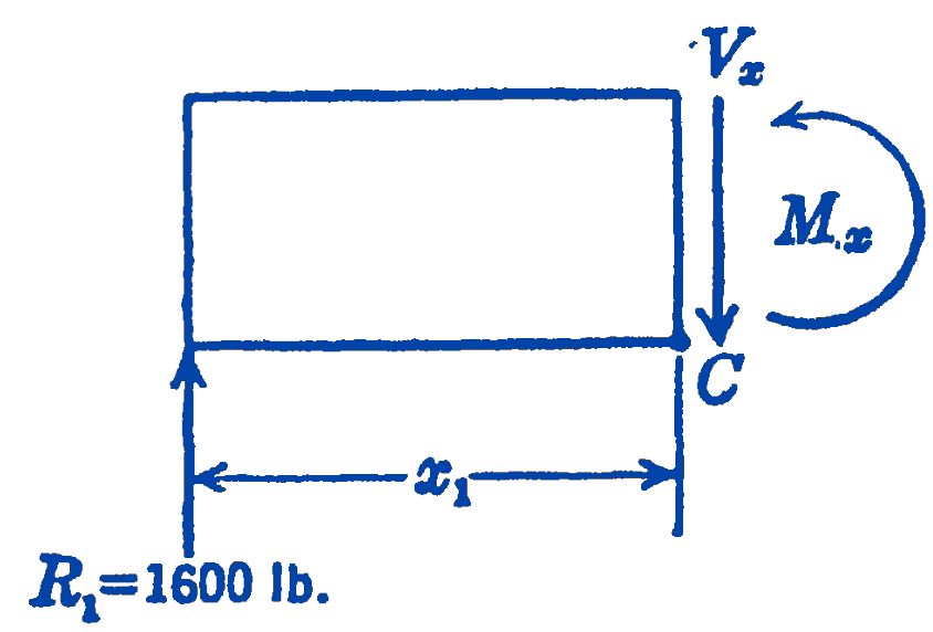
To find the shearing force at any point between \(R_{1}\) and the 1000-lb load, a free-body diagram (Fig. 5) of the portion of the beam to the left of section \(C\) is drawn:
\[ \begin{aligned} \sum F_{y} & =0=1600-V_{x} ; \quad V_{x}=1600\ \mathrm{lb} \\ \sum M_{c} & =0=M_{x}-1600 x_{1} ; \\ M_{x} & =1600 x_{1}\ \mathrm{ft}\cdot\mathrm{lb} \end{aligned} \]
For the next section of the beam, between the 1000-lb load and the 2000-lb load, we draw a free-body diagram (Fig. 6) of the portion of the beam to the left of section \(D\).
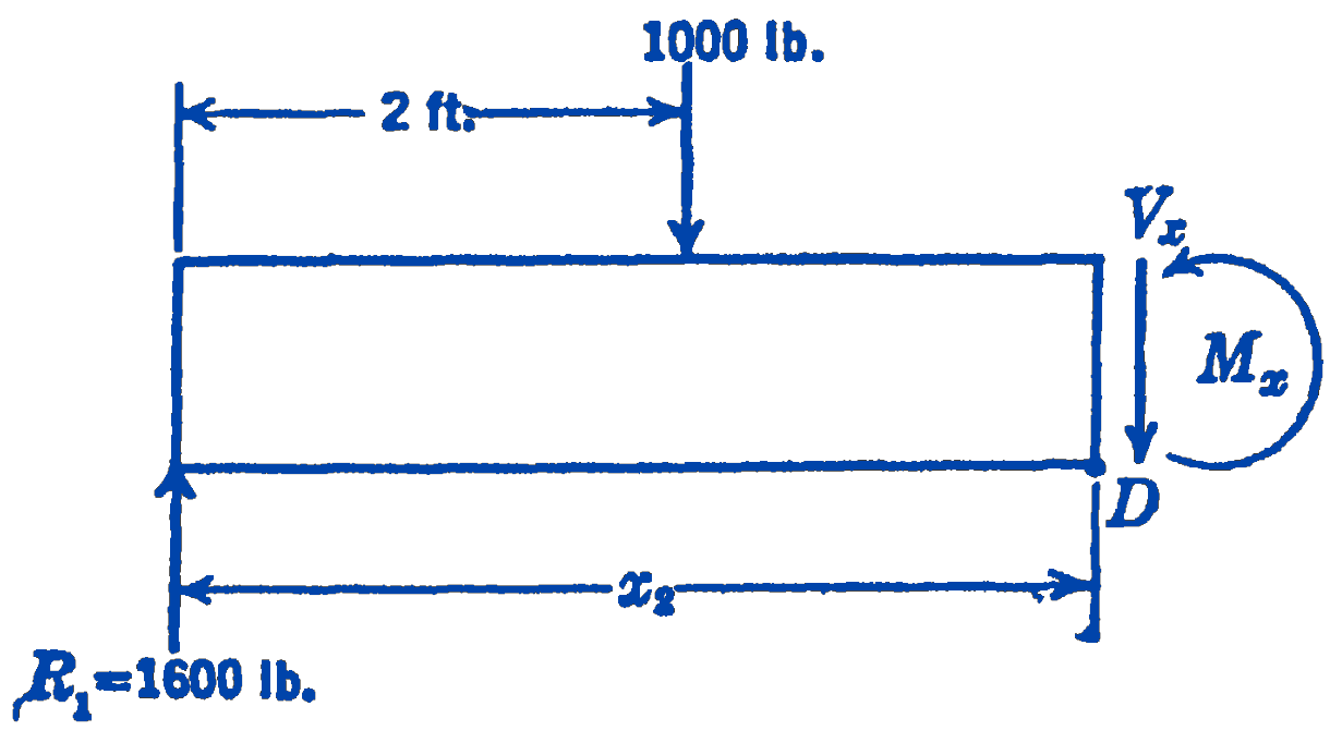
\[ \begin{aligned} \sum F_{y} & =0=1600-1000-V_{x} ; \quad V_{x}=600\ \mathrm{lb} \\ \sum M_{D} & =0=M_{x}-1600 x_{2}+1000\left(x_{2}-2\right) \\ M_{x} & =600 x_{2}+2000\ \mathrm{ft}\cdot\mathrm{lb} \end{aligned} \]
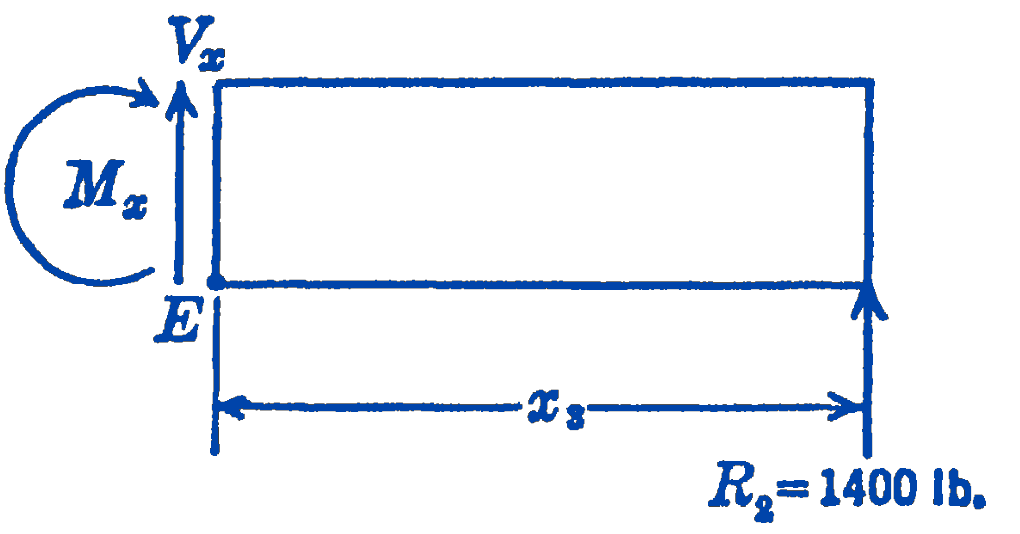
For the rest of the beam, we draw a free-body diagram (Fig. 7) of that portion of the beam to the right of section \(E\) :
\[ \begin{aligned} \sum F_{y}=0 & =1400+V_{x} ; \quad V_{x}=-1400\ \mathrm{lb} \\ \sum M_{B} & =0=1400 x_{3}-M_{x} ; \quad M_{x}=1400 x_{3}\ \mathrm{ft}\cdot\mathrm{lb} \end{aligned} \]
Note that in all of the free-body diagrams the unknown shearing force and bending moments have been shown in the positive direction. In writing the equations of statics, the usual sign conventions have been used.
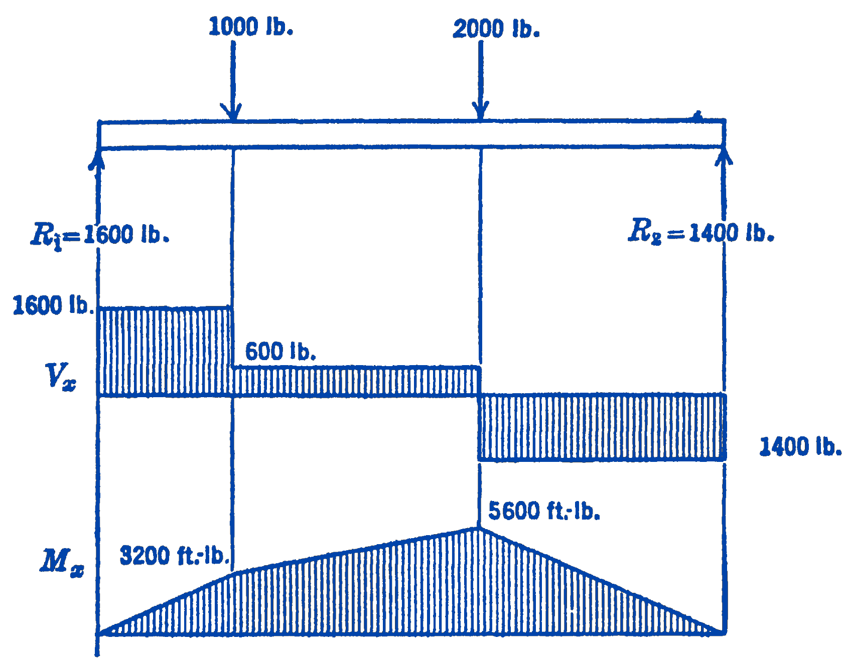
The shearing force and the bending moment diagrams can now be drawn for the whole beam as follows (Fig. 8):
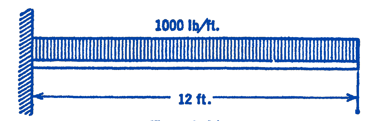
Example 2. Draw the shearing force and bending moment diagrams for the cantilever beam with the uniformly distributed load shown in Fig. 9.
Solution. From the free-body diagram of the entire beam, the reaction force and the reaction moment can be determined (Fig. 10):
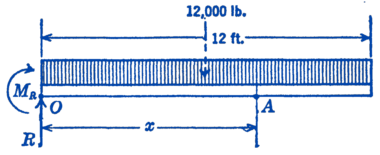
\[ \begin{aligned} \sum M_{0} & =0=-(12,000)(6)-M_{R} \\ M_{R} & =-72,000\ \mathrm{ft}\cdot\mathrm{lb} \\ \sum F_{y} & =0=R-12,000 ; \quad R=12,000\ \mathrm{lb} \end{aligned} \]
To find the shearing force and the bending moment at any point in the beam, we draw a free-body diagram of the portion of the beam to the left of the section \(A\), located a distance \(x\) from the left end of the beam (Fig. 11):
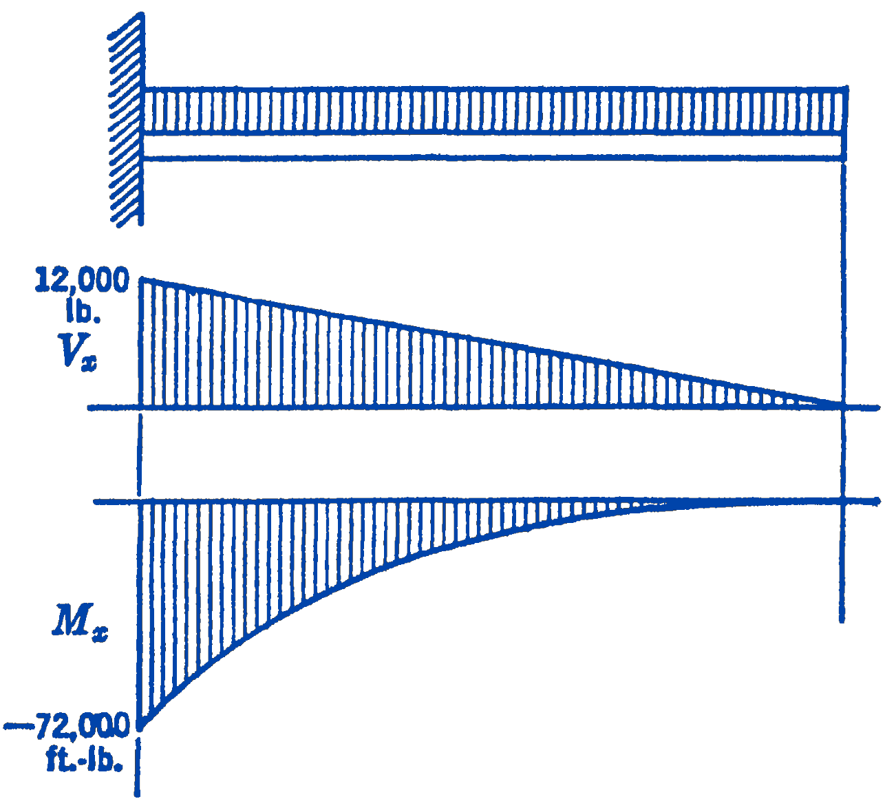
\[ \begin{aligned} \sum F_{y} & =0=12,000-1000 x-V_{x} \\ V_{x} & =12,000-1000 x\ \mathrm{lb} \\ \sum M_{A} & =0=M_{x}+(1000 x)\left(\frac{x}{2}\right)+72,000-12,000 x \\ M_{x} & =12,000 x-500 x^{2}-72,000\ \mathrm{ft}\cdot\mathrm{lb} \end{aligned} \]
Plotting these expressions gives (Fig. 12):
For this problem, it would have been better to have measured \(x\) from the right end of the beam, and to have drawn a free-body diagram of that portion of the section (Fig. 13). This would have eliminated the necessity of determining the beam reactions:
\[ \begin{aligned} & \sum F_{x}=0=V_{x}-1000 x ; \quad V_{x}=1000 x \\ & \sum M_{\Delta}^{x}=0=-M_{x}-500 x^{2} ; \quad M_{x}=-500 x^{2} \end{aligned} \]
It will be seen that these expressions give the same shearing force and bending moment diagrams as found above.
6.11.1 PROBLEMS
For the following beams, draw shearing force and bending moment diagrams, giving numerical values at various significant points :
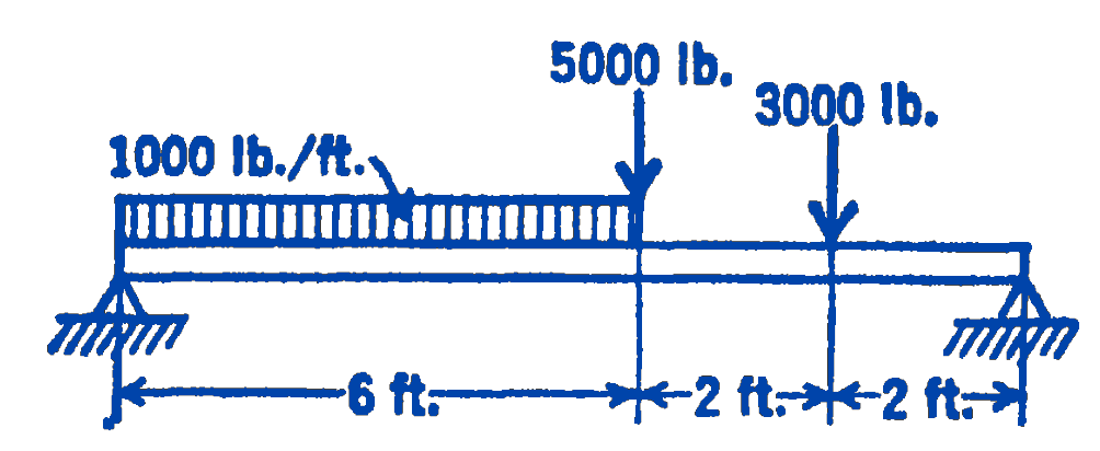
1.
Answer
\(M_{\text {max }}=20,700 \ \mathrm{ft}\cdot\mathrm{lb}\)
2.
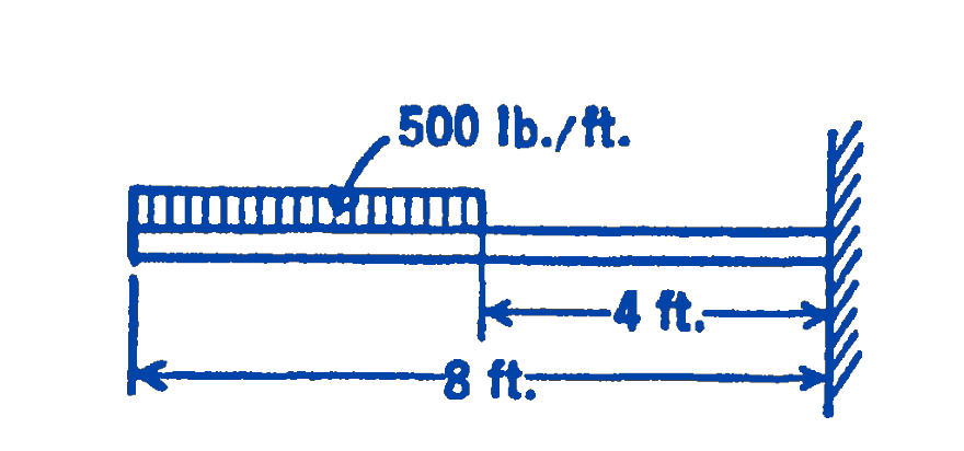
Answer
\(M_{\max }=-12,000 \ \mathrm{ft}\cdot\mathrm{lb}\)
3.
Answer
\(M_{\text {max }}=22,800 \ \mathrm{ft}\cdot\mathrm{lb}\)
4.
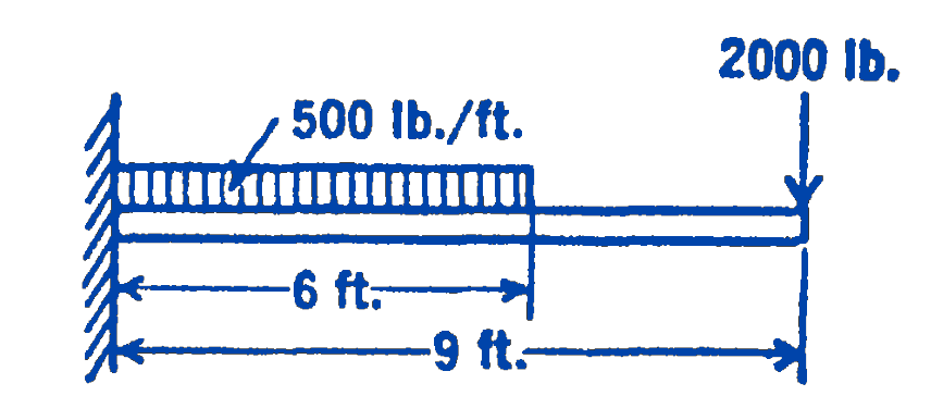
Answer
\(M_{\text {max }}=-27,000 \ \mathrm{ft}\cdot\mathrm{lb}\)
5.
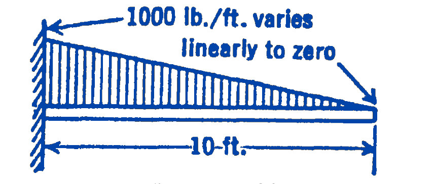
Answer
\(M_{\text {max }}=-16,670 \ \mathrm{ft}\cdot\mathrm{lb}\)
6.
Answer
\(M_{\max }=6,480 \ \mathrm{ft}\cdot\mathrm{lb}\)