Two random variables, \(X_{1}\) and \(X_{2}\) , are said to be jointly distributed if they are defined as functions on the same probability space. It is then possible to make joint probability statements about \(X_{1}\) and \(X_{2}\) (that is, probability statements about the simultaneous behavior of the two random variables). In this section we introduce the notions used to describe the joint probability law of jointly distributed random variables.
The joint probability function, denoted by \(P_{X_{1}, X_{2}}[\cdot]\) of two jointly distributed random variables, is defined for every Borel set \(B\) of 2-tuples of real numbers by
\[P_{X_{1}, X_{2}}[B]=P\left[\left\{s \text { in } S: \ \left(X_{1}(s), X_{2}(s)\right) \text { is in } B\right\}\right], \tag{5.1}\]
in which \(S\) denotes the sample description space on which the random variables \(X_{1}\) and \(X_{2}\) are defined and \(P[\cdot]\) denotes the probability function defined on \(S\) . In words, \(P_{X_{1}, X_{2}}[B]\) represents the probability that the 2-tuple ( \(X_{1}, X_{2}\) ) of observed values of the random variables will lie in the set \(B\) . For brevity, we usually write
\[P_{X_{1}, X_{2}}[B]=P\left[\left(X_{1}, X_{2}\right) \text { is in } B\right], \tag{5.2}\]
instead of (5.1). However, it should be kept constantly in mind that the right-hand side of (5.2) is without mathematical content of its own; rather, it is an intuitively meaningful concise way of writing the right-hand side of (5.1) .
It is useful to think of the joint probability function \(P_{X_{1}, X_{2}}[\cdot]\) of two jointly distributed random variables \(X_{1}\) and \(X_{2}\) as representing the distribution of a unit amount of probability mass over a 2-dimensional plane on which rectangular coordinates have been marked off, as in Fig. 7A of Chapter 4, so that to any point in the plane there corresponds a 2-tuple \(\left(x_{1}^{\prime}, x_{2}^{\prime}\right)\) of real numbers representing it. For any Borel set \(B\) of 2-tuples \(P_{X_{1}, X_{2}}[B]\) represents the amount of probability mass distributed over the set \(B\) .
We are particularly interested in knowing the value \(P_{X_{1}, X_{2}}[B]\) for sets \(B\) , which are combinatorial product sets in the plane. A set \(B\) is called a combinatorial product set if it is of the form \(B=\left\{\left(x_{1}, x_{2}\right): x_{1}\right.\) is in \(B_{1}\) and \(x_{2}\) is in \(\left.B_{2}\right\}\) for some Borel sets \(B_{1}\) and \(B_{2}\) of real numbers. If \(B\) is of this form, we then write, for brevity, \(P_{X_{1}, x_{2}}[B]=P\left[X_{1}\right.\) is in \(B_{1}, X_{2}\) is in \(\left.B_{2}\right]\) .
In order to know the joint probability function \(P_{X_{1}, X_{2}}[B]\) for all Borel sets \(B\) of 2-tuples, it suffices to know it for all infinite rectangle sets \(B_{x_{1}, x_{2}}\) , where, for any two real numbers \(x_{1}\) and \(x_{2}\) , we define the “infinite rectangle” set
\[B_{x_{1}, x_{2}}=\left\{\left(x_{1}^{\prime}, x_{2}^{\prime}\right): \quad x_{1}^{\prime} \leq x_{1}, x_{2}^{\prime} \leq x_{2}\right\} \tag{5.3}\]
as the set consisting of all 2-tuples \(\left(x_{1}^{\prime}, x_{2}^{\prime}\right)\) whose first component \(x_{1}^{\prime}\) is less than the specified real number \(x_{1}\) and whose second component \(x_{2}^{\prime}\) is less than the specified real number \(x_{2}\) . To specify the joint probability function of \(X_{1}\) and \(X_{2}\) , it suffices to specify the joint distribution function \(F_{X_{1}, X_{2}}(.,.)\) , of the random variables \(X_{1}\) and \(X_{2}\) , defined for all real numbers \(x_{1}\) and \(x_{2}\) by the equation
\[F_{X_{1}, X_{2}}\left(x_{1}, x_{2}\right)=P\left[X_{1} \leq x_{1}, X_{2} \leq x_{2}\right]=P_{X_{1}, X_{2}}\left[B_{x_{1}, x_{2}}\right]. \tag{5.4}\]
In words, \(F_{X_{1}, X_{2}}\left(x_{1}, x_{2}\right)\) represents the probability that the simultaneous observation \(\left(X_{1}, X_{2}\right)\) will have the property that \(X_{1} \leq x_{1}\) and \(X_{2} \leq x_{2}\) .
In terms of the probability mass distributed over the plane of Fig. 7A of Chapter 4, \(F_{X_{1}, X_{2}}\left(x_{1}, x_{2}\right)\) represents the amount of mass in the “infinite rectangle” \(B_{x_{1}, x_{2}}\) .
The reader should verify for himself the following important formula [compare (7.3) of Chapter 4]: for any real numbers \(a_{1}, a_{2}, b_{1}\) , and \(b_{2}\) , such that \(a_{1} \leq b_{1}, a_{2} \leq b_{2}\) , the probability \(P\left[a_{1}
\begin{align} P\left[a_{1}
It is important to note that from a knowledge of the joint distribution function \(F_{X_{1}, X_{2}}(.,.)\) of two jointly distributed random variables one may obtain the distribution functions \(F_{X_{1}}(\cdot)\) and \(F_{X_{2}}(\cdot)\) of each of the random variables \(X_{1}\) and \(X_{2}\) . We have the formula for any real number \(x_{1}\) :
\begin{align} F_{X}\left(x_{1}\right) & =P\left[X_{1} \leq x_{1}\right]=P\left[X_{1} \leq x_{1}, X_{2}<\infty\right] \tag{5.6}\\ & =\lim _{x_{2} \rightarrow \infty} F_{X_{1}, X_{2}}\left(x_{1}, x_{2}\right)=F_{X_{1}, X_{2}}\left(x_{1}, \infty\right). \end{align}
Similarly, for any real number \(x_{2}\)
\[F_{X_{2}}\left(x_{2}\right)=\lim _{x_{1} \rightarrow \infty} F_{X_{1}, X_{2}}\left(x_{1}, x_{2}\right)=F_{X_{1}, X_{2}}\left(\infty, x_{2}\right). \tag{5.7}\]
In terms of the probability mass distributed over the plane by the joint distribution function \(F_{X_{1}, X_{2}}(.,.)\) , the quantity \(F_{X_{1}}\left(x_{1}\right)\) is equal to the amount of mass in the half-plane that consists of all 2-tuples \(\left(x_{1}^{\prime}, x_{2}^{\prime}\right)\) that are to the left of, or on, the line with equation \(x_{1}^{\prime}=x_{1}\) .
The function \(F_{X_{1}}(\cdot)\) is called the marginal distribution function of the random variable \(X_{1}\) corresponding to the joint distribution function \(F_{X_{1}, X_{2}}(.,.)\) . Similarly, \(F_{X_{2}}(\cdot)\) is called the marginal distribution function of \(X_{2}\) corresponding to the joint distribution function \(F_{X_{1}, X_{2}}(.,.)\)
We next define the joint probability mass function of two random variables \(X_{1}\) and \(X_{2}\) , denoted by \(p_{X_{1}, X_{2}}(.,.)\) , as a function of 2 variables, with value, for any real numbers \(x_{1}\) and \(x_{2}\) . \begin{align} p_{X_{1}, X_{2}}\left(x_{1}, x_{2}\right) & =P\left[X_{1}=x_{1}, X_{2}=x_{2}\right] \tag{5.8}\\ & =P_{X_{1}, X_{2}}\left[\left\{\left(x_{1}^{\prime}, x_{2}^{\prime}\right): x_{1}^{\prime}=x_{1}, x_{2}^{\prime}=x_{2}\right\}\right]. \end{align}
It may be shown that there is only a finite or countably infinite number of 2-tuples \(\left(x_{1}, x_{2}\right)\) at which \(p_{X_{1}, X_{2}}\left(x_{1}, x_{2}\right)>0\) . The jointly distributed random variables \(X_{1}\) and \(X_{2}\) are said to be jointly discrete if the sum of the joint probability mass function over the points \(\left(x_{1}, x_{2}\right)\) where \(p_{X_{1}, X_{2}}\left(x_{1}, x_{2}\right)\) is positive is equal to 1. If the random variables \(X_{1}\) and \(X_{2}\) are jointly discrete , then they are individually discrete, with individual probability mass functions, for any real numbers \(x_{1}\) and \(x_{2}\) .
\begin{align} & p_{X_{1}}\left(x_{1}\right) =\sum_{\substack{\text { over all } x_{2} \text { such that } \\ p_{X_{1}, X_{2}}(x_{2}, x_{2}) >0}} p_{X_{1}, X_{2}}\left(x_{1}, x_{2}\right) \\ & p_{X_{2}}\left(x_{2}\right) =\sum_{\substack{\text { over all } x_{2} \text { such that } \\ p_{X_{1}, X_{2}}(x_{2}, x_{2}) >0}} p_{X_{1}, X_{2}}\left(x_{1}, x_{2}\right). \tag{5.9}\\ \end{align}
Two jointly distributed random variables, \(X_{1}\) and \(X_{2}\) , are said to be jointly continuous if they are specified by a joint probability density function.
Two jointly distributed random variables, \(X_{1}\) and \(X_{2}\) , are said to be specified by a joint probability density function if there is a nonnegative Borel function \(f_{X_{1}, X_{2}}(.,.)\) , called the joint probability density of \(X_{1}\) and \(X_{2}\) , such that for any Borel set \(B\) of 2-tuples of real numbers the probability \(P\left[\left(X_{1}, X_{2}\right)\right.\) is in \(\left.B\right]\) may be obtained by integrating \(f_{X_{1}, X_{2}}(.,.)\) over \(B\) ; in symbols,
\[P_{X_{1}, X_{2}}[B]=P\left[\left(X_{1}, X_{2}\right) \text { is in } B\right]=\int_{B} \int_{B} f_{X_{1}, X_{2}}\left(x_{1}^{\prime}, x_{2}^{\prime}\right) dx_{1}^{\prime} dx_{2}^{\prime}. \tag{5.10}\]
By letting \(B=B_{x_{1}, x_{2}}\) in (5.10), it follows that the joint distribution function for any real numbers \(x_{1}\) and \(x_{2}\) may be given by
\[F_{X_{1}, X_{2}}\left(x_{1}, x_{2}\right)=\int_{-\infty}^{x_{1}} d x_{1}^{\prime} \int_{-\infty}^{x_{2}} d x_{2}^{\prime} f_{X_{1}, X_{2}}\left(x_{1}^{\prime}, x_{2}^{\prime}\right). \tag{5.11}\]
Next, for any real numbers \(a_{1}, b_{1}, a_{2}, b_{2}\) , such that \(a_{1} \leq b_{1}, a_{2} \leq b_{2}\) , one may verify that
\[P\left[a_{1}
The joint probability density function may be obtained from the joint distribution function by routine differentiation, since
\[f_{X_{1}, X_{2}}\left(x_{1}, x_{2}\right)=\frac{\partial^{2}}{\partial x_{1} \partial x_{2}} F_{X_{1}, X_{2}}\left(x_{1}, x_{2}\right) \tag{5.13}\]
at all 2-tuples \(\left(x_{1}, x_{2}\right)\) , where the partial derivatives on the right-hand side of (5.13) are well defined.
If the random variables \(X_{1}\) and \(X_{2}\) are jointly continuous, then they are individually continuous, with individual probability density functions for any real numbers \(x_{1}\) and \(x_{2}\) given by
\begin{align} & f_{X_{1}}\left(x_{1}\right)=\int_{-\infty}^{\infty} f_{X_{1}, X_{2}}\left(x_{1}, x_{2}\right) d x_{2} \\ & f_{X_{2}}\left(x_{2}\right)=\int_{-\infty}^{\infty} f_{X_{1}, X_{2}}\left(x_{1}, x_{2}\right) d x_{1} . \tag{5.14} \end{align}
The reader should compare (5.14) with (3.4) .
To prove (5.14), one uses the fact that by (5.6), (5.7), and (5.11),
\begin{align} & F_{X_{1}}\left(x_{1}\right)=\int_{-\infty}^{x_{1}} d x_{1}^{\prime} \int_{-\infty}^{\infty} d x_{2}^{\prime} f_{X_{1}, X_{2}}\left(x_{1}^{\prime}, x_{2}^{\prime}\right) \\ & F_{X_{2}}\left(x_{2}\right)=\int_{-\infty}^{x_{2}} d x_{2}^{\prime} \int_{-\infty}^{\infty} d x_{1}^{\prime} f_{X_{1}, X_{2}}\left(x_{1}^{\prime}, x_{2}^{\prime}\right). \end{align}
The foregoing notions extend at once to the case of \(n\) random variables. We list here the most important notations used in discussing \(n\) jointly distributed random variables \(X_{1}, X_{2}, \ldots, X_{n}\) . The joint probability function for any Borel set \(B\) of \(n\) -tuples is given by
\[P_{X_{1}, X_{2}, \ldots, X_{n}}[B]=P\left[\left(X_{1}, X_{2}, \ldots, X_{n}\right) \text { is in } B\right]. \tag{5.15}\] The joint distribution function for any real numbers \(x_{1}, x_{2}, \ldots, x_{n}\) is given by \[F_{X_{1}, X_{2}, \ldots, X_{n}}\left(x_{1}, x_{2}, \ldots, x_{n}\right) =P\left[X_{1} \leq x_{1}, X_{2} \leq x_{2}, \ldots, X_{n} \leq x_{n}\right]. \tag{5.16}\] The joint probability density function (if the derivative below exists) is given by
\begin{align} f_{X_{1}, X_{2}, \ldots, X_{n}}\left(x_{1}, x_{2}, \ldots, x_{n}\right) =\frac{\partial^{n}}{\partial x_{1} \partial x_{2} \cdots \partial x_{n}} F_{X_{1}, X_{2}, \ldots, X_{n}}\left(x_{1}, x_{2}, \ldots, x_{n}\right). \tag{5.17} \end{align}
The joint probability mass function is given by \begin{align} p_{X_{1}, X_{2}, \ldots, X_{n}}\left(x_{1}, x_{2}, \ldots, x_{n}\right) = P\left[X_{1}=x_{1}, X_{2}=x_{2}, \ldots, X_{n}=x_{n}\right]. \tag{5.18} \end{align} A discrete joint probability law is specified by its probability mass function: for any Borel set \(B\) of \(n\) -tuples
\[P_{X_{1}, X_{2}, \ldots, X_{n}}[B] \tag{5.19} \\ =\sum_{\substack{\text { over all }\left(x_{1}, x_{2}, \ldots, x_{n}\right) \text { in } B \text { such that } \\ p_{X_{1}, X_{2}, \ldots, X_{n}} \left(x_{1}, x_{2}, \ldots, x_{n}\right)>0}} p_{X_{1}, X_{2}, \ldots, X_{n}}\left(x_{1}, x_{2}, \ldots, x_{n}\right).\]
A continuous joint probability law is specified by its probability density function: for any Borel set \(B\) of \(n\) -tuples
\begin{align} & P_{X_{1}, X_{2}, \ldots, X_{n}}[B] \tag{5.20}\\ & \quad=\iint_{B} \cdots \int f_{X_{1}, X_{2},\ldots, X_{n}} \left(x_{1}, x_{2}, \ldots, x_{n}\right) d x_{1} d x_{2} \cdots d x_{n} . \end{align}
The individual (or marginal ) probability law of each of the random variables \(X_{1}, X_{2}, \ldots, X_{n}\) may be obtained from the joint probability law. In the continuous case, for any \(k=1,2, \ldots, n\) and any fixed number \(x_{k}^{0}\) ,
\begin{align} f_{X_{k}}\left(x_{k}^{0}\right)=\int_{-\infty}^{\infty} d x_{1} \cdots \int_{-\infty}^{\infty} d x_{k-1} & \int_{-\infty}^{\infty} d x_{k+1} \cdots \int_{-\infty}^{\infty} d x_{n} \tag{5.21}\\ & f_{X_{1}, X_{2}, \ldots, X_{n}}\left(x_{1}, \ldots, x_{k}^{0}, x_{k+1}, \cdots x_{n}\right). \end{align}
An analogous formula may be written in the discrete case for \(p_{x_{k}}\left(x_{k}^{0}\right)\) .
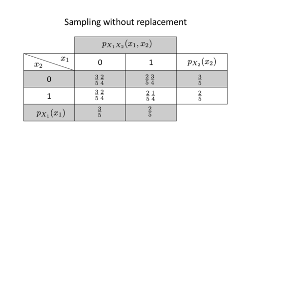
Example 5A . Jointly discrete random variables . Consider a sample of size 2 drawn with replacement (without replacement) from an urn containing two white, one black, and two red balls. Let the random variables \(X_{1}\) and \(X_{2}\) be defined as follows; for \(k=1,2, X_{k}=1\) or 0, depending on whether the ball drawn on the \(k\) th draw is white or nonwhite. (i) Describe the joint probability law of \(\left(X_{1}, X_{2}\right)\) . (ii) Describe the individual (or marginal) probability laws of \(X_{1}\) and \(X_{2}\) .
Solution
The random variables \(X_{1}\) and \(X_{2}\) are clearly jointly discrete. Consequently, to describe their joint probability law, it suffices to state their joint probability mass function \(p_{x_{1}, x_{2}}\left(x_{1}, x_{2}\right)\) . Similarly, to describe their individual probability laws, it suffices to describe their individual probability mass functions \(p_{X_{1}}\left(x_{1}\right)\) and \(p_{X_{2}}\left(x_{2}\right)\) . These functions are conveniently presented in the following tables:

Example 5B . Jointly continuous random variables . Suppose that at two points in a room (or on a city street or in the ocean) one measures the intensity of sound caused by general background noise. Let \(X_{1}\) and \(X_{2}\) be random variables representing the intensity of sound at the two points. Suppose that the joint probability law of the sound intensities, \(X_{1}\) and \(X_{2}\) , is continuous, with the joint probability density function given by
\begin{align} f_{X_{1}, X_{2}}(x_{1}, x_{2}) = \begin{cases} x_{1} x_{2} \exp\left(-\frac{1}{2}(x_{1}^{2} + x_{2}^{2})\right), & \text{if } x_{1} > 0 \text{ and } x_{2} > 0 \\ 0, & \text{otherwise.} \end{cases} \end{align}
Find the individual probability density functions of \(X_{1}\) and \(X_{2}\) . Further, find \(P\left[X_{1} \leq 1, X_{2} \leq 1\right]\) and \(P\left[X_{1}+X_{2} \leq 1\right]\) .
Solution
By (5.14) , the individual probability density functions are given by \begin{align} & f_{X_{1}}\left(x_{1}\right)=\int_{0}^{\infty} x_{1} x_{2} \exp \left[-\frac{1}{2}\left(x_{1}^{2}+x_{2}^{2}\right)\right] d x_{2}=x_{1} \exp \left(-\frac{1}{2} x_{1}^{2}\right) \\ & f_{X_{2}}\left(x_{2}\right)=\int_{0}^{\infty} x_{1} x_{2} \exp \left[-\frac{1}{2}\left(x_{1}^{2}+x_{2}^{2}\right)\right] d x_{1}=x_{2} \exp \left(-\frac{1}{2} x_{2}^{2}\right). \end{align}
Note that the random variables \(X_{1}\) and \(X_{2}\) are identically distributed. Next, the probability that each sound intensity is less than or equal to 1 is given by \begin{align} P\left[X_{1} \leq 1, X_{2} \leq 1\right] & =\int_{-\infty}^{1} \int_{-\infty}^{1} f_{X_{1}, X_{2}}\left(x_{1}, x_{2}\right) d x_{1} d x_{2} \\[2mm] & =\left(\int_{0}^{1} x_{1} e^{-1 / 2 x_{1}^{2}} d x_{1}\right)\left(\int_{0}^{1} x_{2} e^{-1 / 2 x_{2}^{2}} d x_{2}\right)=0.1548. \end{align}
The probability that the sum of the sound intensities is less than 1 is given by \begin{align} P\left[X_{1}+X_{2} \leq 1\right] & =\displaystyle\iint_{\left\{\left(x_{1}, x_{2}\right):x_{1}+x_{2} \leq 1 \right.} f\left(x_{1}, x_{2}\right) d x_{1} d x_{2} \\ & =\int_{0}^{1} d x_{1} x_{1} e^{- 1 / 2 x_{1}^{2}} \int_{0}^{1-x_{1}} d x_{2} x_{2} e^{-1 / 2 x_{2}^{2}}=0.2433. \end{align}
Example 5C . The maximum noise intensity . Suppose that at five points in the ocean one measures the intensity of sound caused by general background noise (the so-called ambient noise). Let \(X_{1}, X_{2}, X_{3}, X_{4}\) , and \(X_{5}\) be random variables representing the intensity of sound at the various points. Suppose that their joint probability law is continuous, with joint probability density function given by
\begin{align} f_{X_{1}, X_{2}, X_{3}, X_{4}, X_{5}}(x_{1}, x_{2}, x_{3}, x_{4}, x_{5}) = \begin{cases} x_{1} x_{2} x_{3} x_{4} x_{5} \exp\left(-\frac{1}{2}\left(x_{1}^{2} + x_{2}^{2} + x_{3}^{2} + x_{4}^{2} + x_{5}^{2}\right)\right), & \text{if } 0 \leq x_{1}, x_{2}, x_{3}, x_{4}, x_{5} \\ 0, & \text{otherwise.} \end{cases} \end{align}
Define \(Y\) as the maximum intensity; in symbols, \(Y=\) maximum \(\left(X_{1}, X_{2}, X_{3}, X_{4}, X_{5}\right)\) . For any positive number \(y\) the probability that \(Y\) is less than or equal to \(y\) is given by
\begin{align} P[Y \leq y] & =P\left[X_{1} \leq y, X_{2} \leq y, \ldots, X_{5} \leq y\right] \\ & =\int_{-\infty}^{y} dx_{1} \int_{-\infty}^{y} d x_{2} \cdots \int_{-\infty}^{y} d x_{5} f_{X_{1}, X_{2}, X_{3}, X_{4}, X_{5}}\left(x_{1}, x_{2}, \cdots, x_{5}\right) \\ & =\left(\int_{0}^{y} x e^{-1 / 2 x^{2}} dx\right)^{5}=\left(1-e^{-1 / 2 y^{2}}\right)^{5}. \end{align}
Theoretical Exercise
5.1 . Multivariate distributions with given marginal distributions . Let \(f_{1}(\cdot)\) and \(f_{2}(\cdot)\) be two probability density functions. An infinity of joint probability densities \(f(.,.)\) exist, of which \(f_{1}(\cdot)\) and \(f_{2}(\cdot)\) are the marginal probability density functions [that is, such that (3.4) holds]. One method of constructing \(f(.,.)\) is given by (3.9) ; verify this assertion. Show that another method of constructing a joint probability density function \(f(.,.)\) , with given marginal probability density functions \(f_{1}(\cdot)\) and \(f_{2}(\cdot)\) , is by defining for a given constant \(a\) , such that \(|a| \leq 1\) ,
\[f\left(x_{1}, x_{2}\right)=f_{1}\left(x_{1}\right) f_{2}\left(x_{2}\right)\left\{1+a\left[2 F_{1}\left(x_{1}\right)-1\right]\left[2 F_{2}\left(x_{2}\right)-1\right]\right\} \tag{5.22}\]
in which \(F_{1}(\cdot)\) and \(F_{2}(\cdot)\) are the distribution functions corresponding to \(f_{1}(\cdot)\) and \(f_{2}(\cdot)\) , respectively. Show that the distribution function \(F(.,.)\) corresponding to \(f(.,.)\) is given by
\[F\left(x_{1}, x_{2}\right)=F_{1}\left(x_{1}\right) F_{2}\left(x_{2}\right)\left\{1+a\left[1-F_{1}\left(x_{1}\right)\right]\left[1-F_{2}\left(x_{2}\right)\right]\right\} \tag{5.23}\]
Equations (5.22) and (5.23) are due to E. J. Gumbel, “Distributions à plusieurs variables dont les marges sont données”, \(C\) . R. Acad. Sci. Paris, Vol. 246 (1958), pp. 2717–2720.
Exercises
In exercises 5.1 to 5.3 consider a sample of size 3 drawn with replacement (without replacement) from an urn containing (i) 1 white and 2 black balls,
(ii) 1 white, 1 black, and 1 red ball. For \(k=1,2,3\) let \(X_{k}=1\) or 0 depending on whether the ball drawn on the \(k\) th draw is white or nonwhite.
5.1 . Describe the joint probability law of \(\left(X_{1}, X_{2}, X_{3}\right)\) .
Answer
| (i), (ii) | \(\left(x_{1}, x_{2}, x_{3}\right)\) | \(p_{X_{1}, X_{2}, X_{3}}\left(x_{1}, x_{2}, x_{3}\right)\) |
|---|---|---|
| with | \((0,0,0)\) | \(\left(\frac{2}{3}\right)^{3}\) |
| \((1,0,0),(0,1,0),(0,0,1)\) | \(\frac{1}{3}\left(\frac{2}{3}\right)^{2}\) | |
| \((1,1,0),(1,0,1),(0,1,1)\) | \(\frac{2}{3}\left(\frac{1}{3}\right)^{2}\) | |
| \((1,1,1)\) | \(\left(\frac{1}{3}\right)^{3}\) | |
| otherwise | 0; | |
| without, | \(\quad(1,0,0),(0,1,0),(0,0,1)\) | \(\frac{1}{3}\) |
| otherwise | 0. |
5.2 . Describe the individual (marginal) probability laws of \(X_{1}, X_{2}, X_{3}\) .
5.3 . Describe the individual probability laws of the random variables \(Y_{1}, Y_{2}\) , and \(Y_{3}\) , in which \(Y_{1}=X_{1}+X_{2}+X_{3}, Y_{2}=\operatorname{maximum}\left(X_{1}, X_{2}, X_{3}\right)\) . and \(Y_{3}=\operatorname{minimum}\left(X_{1}, X_{2}, X_{3}\right)\) .
Answer
With, \(p_{Y_{1}}(y)=\left(\begin{array}{l}3 \\ y\end{array}\right)\left(\frac{1}{3}\right)^{y}\left(\frac{2}{3}\right)^{3-y} \quad\) if \(y=0,1,2,3 ;=0\) otherwise;
\[\begin{array}{lll} p_{Y_{2}}(y)=\left(\frac{2}{3}\right)^{3} & \text { if } y=0 ;=1-\left(\frac{2}{3}\right)^{3} & \text { if } y=1 ;=0 \text { otherwise; } \\ p_{Y_{3}}(y)=1-\left(\frac{1}{3}\right)^{3} & \text { if } y=0 ;=\left(\frac{1}{3}\right)^{3} & \text { if } y=1 ;=0 \text { otherwise; } \end{array}\]
without, \(p_{Y_{1}}(1)=p_{Y_{2}}(1)=p_{Y_{3}}(0)=1\) .
In exercises 5.4 to 5.6 consider 2 random variables, \(X_{1}\) and \(X_{2}\) , with joint probability law specified by the joint probability density function
(a) \begin{align} f_{X_{1}, X_{2}}(x_{1}, x_{2}) = \begin{cases} \frac{1}{4}, & \text{if } 0 \leq x_{1} \leq 2 \text{ and } 0 \leq x_{2} \leq 2 \\ 0, & \text{otherwise.} \end{cases} \end{align}
(b) \begin{align} f_{X_{1}, X_{2}}(x_{1}, x_{2}) = \begin{cases} e^{-(x_{1} + x_{2})}, & \text{if } x_{1} \geq 0 \text{ and } x_{2} \geq 0 \\ 0, & \text{otherwise.} \end{cases} \end{align}
5.4 . Find (i) \(P\left[X_{1} \leq 1, X_{2} \leq 1\right]\) , (ii) \(P\left[X_{1}+X_{2} \leq 1\right]\) , (iii) \(P\left[X_{1}+X_{2}>2\right]\) .
5.5 . Find (i) \(P\left[X_{1}<2 X_{2}\right]\) , (ii) \(P\left[X_{1}>1\right]\) , (iii) \(P\left[X_{1}=X_{2}\right]\) .
Answer
(a) (i) \(\frac{3}{4}\) , (ii) \(\frac{1}{2}\) , (iii) 0; (b) (i) \(\frac{2}{3}\) , (ii) \(e^{-1}\) , (iii) 0.
5.6 . Find (i) \(P\left[X_{2}>1 \mid X_{1} \leq 1\right]\) , (ii) \(P\left[X_{1}>X_{2} \mid X_{2}>1\right]\) .
In exercises 5.7 to 5.10 consider 2 random variables, \(X_{1}\) and \(X_{2}\) , with the joint probability law specified by the probability mass function \(p_{X_{1}, X_{2}}(.,.)\) given for all \(x_{1}\) and \(x_{2}\) at which it is positive by (a) Table 5A, (b) Table 5B, in which for brevity we write \(h\) for \(\frac{1}{60}\) .
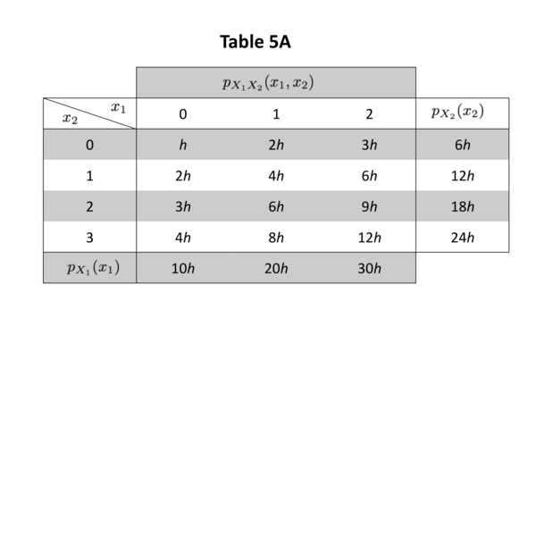
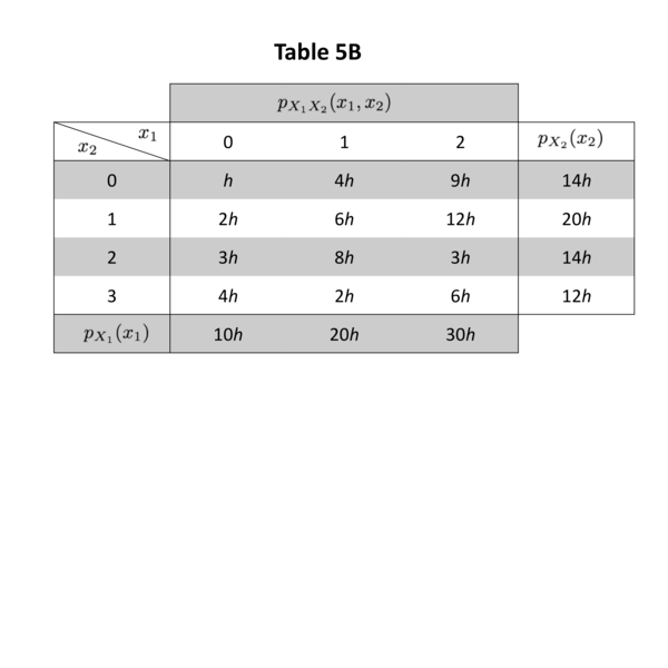
5.7 . Show that the individual probability mass functions of \(X_{1}\) and \(X_{2}\) may be obtained by summing the respective columns and rows as indicated. Are \(X_{1}\) and \(X_{2}\) (i) jointly discrete, (ii) individually discrete?
Answer
Yes.
5.8 . Find (i) \(P\left[X_{1} \leq 1, X_{2} \leq 1\right]\) , (ii) \(P\left[X_{1}+X_{2} \leq 1\right]\) , (iii) \(P\left[X_{1}+X_{2}>2\right]\) .
5.9 . Find (i) \(P\left[X_{1}<2 X_{2}\right]\) , (ii) \(P\left[X_{1}>1\right]\) , (iii) \(P\left[X_{1}=X_{2}\right]\) .
Answer
(a) (i) \(\frac{4}{5}\) , (ii) \(\frac{1}{2}\) , (iii) \(\frac{7}{30}\) ; (b) (i) \(\frac{17}{30}\) , (ii) \(\frac{1}{2}\) , (iii) \(\frac{1}{6}\) .
5.10 . Find (i) \(P\left[X_{1} \geq X_{2} \mid X_{2}>1\right]\) , (ii) \(P\left[X_{1}^{2}+X_{2}^{2} \leq 1\right]\) .