Review: Geometries and Fields

37.1 LECTURE
37.2 REMARKS
37.3 PROTOTYPE EXAMPLES

37.1 LECTURE

37.1.1 Classifying Integral Theorems by Dimension

The Integral theorems deal with geometries $G$ and fields $F$ . Integration pairs them in the form of Stokes theorem $\int_{G} d F = \int_{d G} F$ which involves the boundary $d G$ of $G$ and the exterior derivative $d F$ of $F$ . One can classify the theorems by looking at the dimension $n$ of the underlying space and the dimension $m$ of the object $G$ . In dimension $n$ , there are $n$ theorems:

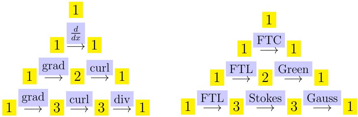
37.1.2 Gradient and Line Integrals

The Fundamental theorem of line integrals is a theorem about the gradient $\nabla f$ . It tells that if $C$ is a curve going from $A$ to $B$ and $f$ is a function (that is a $0$ -form), then

Theorem 1. $\int_{C} \nabla f \cdot d r = f (B) - f (A)$ .

In calculus we write the $1$ -form as a column vector field $\nabla f$ . It actually is a $1$ -form $F = d f$ , a field which attaches a row vector to every point. If the $1$ -form is evaluated at r^{\prime}(t) one gets d f(r(t))(r^{\prime}(t)) which is the matrix product. We integrate then the pull back of the $1$ -form on the interval $[a, b]$ . It is the switch from row vectors to column vectors which leads to the dot product \nabla f(r(t)) \cdot r^{\prime}(t). For closed curves, the line integral is zero. It follows also that integration is path independent.

37.1.3 Curls and Line Integrals: Green’s Connection

Green’s theorem tells that if $G \subset ℝ^{2}$ is a region bound by a curve $C$ having $G$ to the left, then

Theorem 2. $\iint_{G} curl (F) d x d y = \int_{C} F \cdot d r$ .

In the language of forms, $F = P d x + Q d y$ is a $1$ -form and \begin{aligned} d F&=(P_{x} \,d x+P_{y} \,d y) \,d x+(Q_{x} \,d x+Q_{y} \,d y) \,d y\\ &=(Q_{x}-P_{y}) \,d x \,d y \end{aligned} is a $2$ -form. We write this $2$ -form $d F$ as $Q_{x} - P_{y}$ and treat it as a scalar function even so this is not the same as a $0$ -form, which is a scalar function. If $curl (F) = 0$ everywhere in $ℝ^{2}$ then $F$ is a gradient field.

**Figure 1.** Fundamental theorem of line integrals and Green’s theorem.

37.1.4 Surfaces and Line Integrals

Stokes theorem tells that if $S$ is a surface with boundary $C$ oriented to have $S$ to the left and $F$ is a vector field, then

Theorem 3. $\iint_{S} curl (F) \cdot d S = \int_{C} F \cdot d r$ .

In the general frame work, the field $F = P d x + Q d y + R d z$ is a $1$ -form and the $2$ -form \begin{aligned} d F&=(P_{x} \,d x+P_{y} \,d y+P_{z} \,d z) \,d x\\ &\quad +(Q_{x} \,d x+Q_{y} \,d y+Q_{z} \,d z) \,d y\\ &\quad +(R_{x} \,d x+R_{y} \,d y+R_{z} \,d z) \,d z\\ &=(Q_{x}-P_{y}) \,d x \,d y+(R_{y}-Q_{z}) \,d y \,d z+(P_{z}-R_{x}) \,d z \,d x \end{aligned} is written as a column vector field $curl (F) = [R_{y} - Q_{z}, P_{z} - R_{x}, Q_{x} - P_{y}]^{T} .$ To understand the flux integral, we need to see what a bilinear form like $d x d y$ does on the pair of vectors $r_{u}$ , $r_{v}$ . In the case $d x d y$ we have $d x d y (r_{u}, r_{v}) = x_{u} y_{v} - y_{u} x_{v}$ which is the third component of the cross product $r_{u} \times r_{v}$ with $r_{u} = [x_{u}, y_{u}, z_{u}]^{T}$ . Integrating $d F$ over $S$ is the same as integrating the dot product of $curl (F) \cdot r_{u} \times r_{v}$ . Stokes theorem implies that the flux of the curl of $F$ only depends on the boundary of $S$ . In particular, the flux of the curl through a closed surface is zero because the boundary is empty.

**Figure 2.** Stokes theorem and the Gauss theorem.

37.1.5 Gauss Theorem: Sources, Sinks, and the Big Picture

Gauss theorem: if the surface $S$ bounds a solid $E$ in space, is oriented outwards, and $F$ is a vector field, then

Theorem 4. $∭_{E} div (F) d V = \iint_{S} F \cdot d S$ .

Gauss theorem deals with a $2$ -form $F = P d y d z + Q d z d x + R d x d y,$ but because a $2$ -form has three components, we can write it as a vector field $F = [P, Q, R]^{T}$ . We have computed \begin{aligned} d F&=(P_{x} \,d x+P_{y} \,d y+Q_{z} \,d z) \,d y \,d z\\ &\quad +(Q_{x} \,d x+Q_{y} \,d y+Q_{z} \,d z) \,d z \,d x\\ &\quad +(R_{x} \,d x+R_{y} \,d y+R_{z} \,d z) \,d x \,d y, \end{aligned} where only the terms $P_{x} d x d y d z + Q_{y} d y d z d x + R_{z} d z d x d y = (P_{x} + Q_{y} + R_{z}) d x d y d z$ survive which we associate again with the scalar function $div (F) = P_{x} + Q_{y} + R_{z}$ . The integral of a $3$ -form over a $3$ -solid is the usual triple integral. For a divergence free vector field $F$ , the flux through a closed surface is zero. Divergence-free fields are also called incompressible or source free.

37.2 REMARKS

37.2.1 Triplet Trouble: Tensor Types Collide in 3D

We see why the $3$ -dimensional case looks confusing at first. We have three theorems which look very different. This type of confusion is common in science: we put things in the same bucket which actually are different: it is only in $3$ dimensions that $1$ -forms and $2$ -forms can be identified. Actually, more is mixed up: not only are $1$ -forms and $2$ -forms identified, they are also written as vector fields which are $T_{0}^{1}$ tensor fields. From the tensor calculus point of view, we identify the three spaces $T_{0}^{1} (E) = E, T_{1}^{0} (E) = Λ^{1} (E) = E^{*}, and Λ^{2} (E) \subset T_{2}^{0} .$ While we can still always identify vector fields with $1$ -forms, this identification in a general non-flat space will depend on the metric. In $ℝ^{4}$ , the $2$ -forms have dimension $6$ and can no more be written as a vector. One still does. The electro-magnetic $F$ is a $2$ -form in $ℝ^{4}$ which we write as a pair of two time-dependent vector fields, the electric field $E$ and the magnetic field $B$ .

37.2.2 Hilbert Space Harmonization: Merging Geometries and Fields

Geometries and fields are remarkably similar. On geometries, the boundary operation $d$ satisfies $d \circ d = 0$ . On fields the derivative operation $d$ satisfies $d \circ d = 0$ . "Geometries" as well as "fields" come with an orientation: $r_{u} \times r_{v} = - r_{v} \times r_{u}, d x d y = - d y d x .$ The operations $d$ and $d$ look different because calculus deals with smooth things like curves or surfaces leading to generalized functions. In quantum calculus they are thickened up and $d$ , $d$ defined without limit. Fields and geometries then become indistinguishable elements in a Hilbert space. The exterior derivative $d$ has as an adjoint $d = d^{*}$ which is the boundary operator. It is a kind of quantum field theory as $d$ generates while $d^{*}$ destroys a "particle". $d^{2} = d^{2} = 0$ is a "Pauli exclusion".

37.2.3 Dual Forms and Jacobians: A Manifold-Field Marriage

We can spin this further: a $𝒎$ -manifold $S$ is the image of a parametrization $r : G \subset ℝ^{m} \to ℝ^{n}$ . The Jacobian $d r$ is a dual $𝒎$ -form, the exterior product of the $m$ vectors $d r_{u_{1}}$ up to $d r_{u_{m}}$ (think of $m$ column vectors attached to $r (u) \in S$ ). If we take a map $s : S \subset ℝ^{n} \to ℝ^{m}$ and look at $F = d s$ , we can think of it as a $m$ -form $F$ (think of $m$ row vectors attached to each point $x$ in $ℝ^{n}$ ). The map $s$ defines $m \times n$ Jacobian $d s (x)$ , while the Jacobian $d r (u)$ is the $n \times m$ matrix. Cauchy-Binet shows that the flux of $F = d s$ through $r (G) = S$ is the integral $\int_{G} F = \int_{G} \det (d s (r (u)) d r (u)) d u = \int_{S} \det (d s (x) d r (s (x))) .$ If $s (r (u)) = u$ , then this is a geometric functional. So: geometries $G$ can come from maps from a space $A$ to a space $B$ , while fields $F$ can come from maps from $B$ to $A$ . The action integral $\int_{G} F$ generalizes the Polyakov action $\int_{G} \det (d r^{T} d r) = \int_{G} | d r |^{2},$ a case where $F$ and $G$ are dual meaning $s (r (u)) = u$ .

37.3 PROTOTYPE EXAMPLES

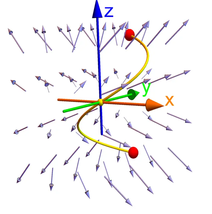
Example 1. Problem: Compute the line integral of $F (x, y, z) = [5 x^{4} + z y, 6 y^{5} + x z, 7 z^{6} + x y]$ along the path $r (t) = [\sin (5 t), \sin (2 t), t^{2} / π^{2}]$ from $t = 0$ to $t = 2 π$ .
Solution: The field is a gradient field $d f$ with $f = x^{5} + y^{6} + z^{7} + x y z$ . We have \begin{aligned} A=r(0)=(0,0,0), \quad B=r(2 \pi)=(0,0,4), \quad f(A)=1, \quad f(B)=4^{7}. \end{aligned} The fundamental theorem of line integrals gives $\int_{C} \nabla f d r = f (B) - f (A) = 4^{7} .$

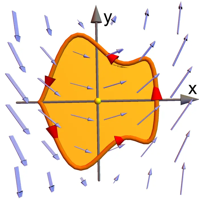
Example 2. Problem: Find the line integral of the vector field $F (x, y) = [x^{4} + \sin (x) + y + 5 x y, 4 x + y^{3}]$ along the cardioid $r (t) = (1 + \sin (t)) [\cos (t), \sin (t)]$ , where $t$ runs from $t = 0$ to $t = 2 π$ .
Solution: We use Green’s theorem. Since $curl (F) = 3 - 5 x$ , the line integral is the double integral $\iint_{G} (3 - 5 x) d x d y .$ We integrate in polar coordinates and get $\int_{0}^{2 π} \int_{0}^{1 + \sin (t)} (3 - 5 r \cos (t)) r d r d t$ which is $9 π / 2$ . One can short cut by noticing that by symmetry $\iint_{G} (- 5 x) d x d y = 0$ , so that the integral is $3$ times the area $\int_{0}^{2 π} (1 + \sin (t))^{2} / 2 d t = 3 π / 2$ of the cardioid.

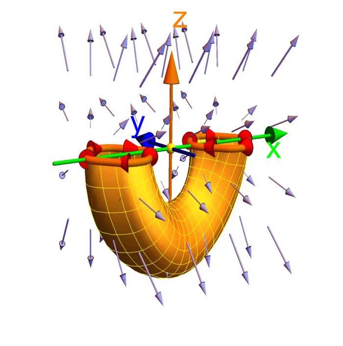
Example 3. Problem: Compute the line integral of $F (x, y, z) = [x^{3} + x y, y, z]$ along the polygonal path $C$ connecting the points $(0, 0, 0)$ , $(2, 0, 0)$ , $(2, 1, 0)$ , $(0, 1, 0)$ .
Solution: The path $C$ bounds a surface $S : r (u, v) = [u, v, 0]$ parameterized on $G = {(x, y) ∣ x \in [0, 2], y \in [0, 1]} .$ By Stokes theorem, the line integral is equal to the flux of $curl (F) (x, y, z) = [0, 0, - x]$ through $S$ . The normal vector of $S$ is $r_{u} \times r_{v} = [1, 0, 0] \times [0, 1, 0] = [0, 0, 1]$ so that \begin{aligned} \iint_{S} \operatorname{curl}(F) \cdot d S&=\int_{0}^{2} \int_{0}^{1}[0,0,-u] \cdot[0,0,1] \,d v \,d u\\ &=\int_{0}^{2} \int_{0}^{1}-u \,d v \,d u\\ &=-2. \end{aligned}

Example 4. Problem: Compute the flux of the vector field $F (x, y, z) = [- x, y, z^{2}]$ through the boundary $S$ of the rectangular box $G = [0, 3] \times [- 1, 2] \times [1, 2] .$ Solution: By the Gauss theorem, the flux is equal to the triple integral of $div (F) = 2 z$ over the box: $\int_{0}^{3} \int_{- 1}^{2} \int_{1}^{2} 2 z d z d y d x = (3 - 0) (2 - (- 1)) (4 - 1) = 27.$