In order to understand how to transform stress components into a new coordinate system in 3D, we first revisit the simpler 2D case. We will approach the 2D transformation differently than before, beginning with the transformation of a vector.

Transformation of a Vector in 2D

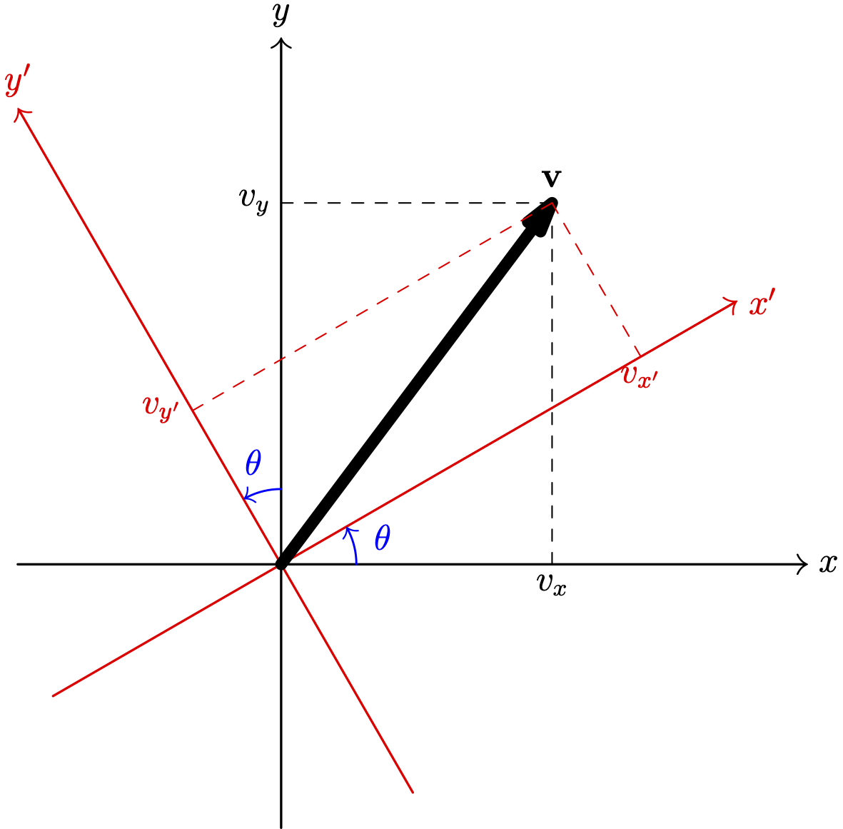
Suppose that we have rotated the coordinate system by an angle \(\theta\). Let’s call the new coordinate system x’y’. We want to see how the components of a vector in a new system can be obtained from its components. That is, if the components of a vector \(\mathbf{v}\) be \(v_x\) and \(v_y\) in the old system and \(v_{x'}\) and \(v_{y'}\) in the new system (see the following figure), we want to express \(v_{x'}\) and \(v_{y'}\) in terms of \(v_x\) and \(v_y\) .

First Approach

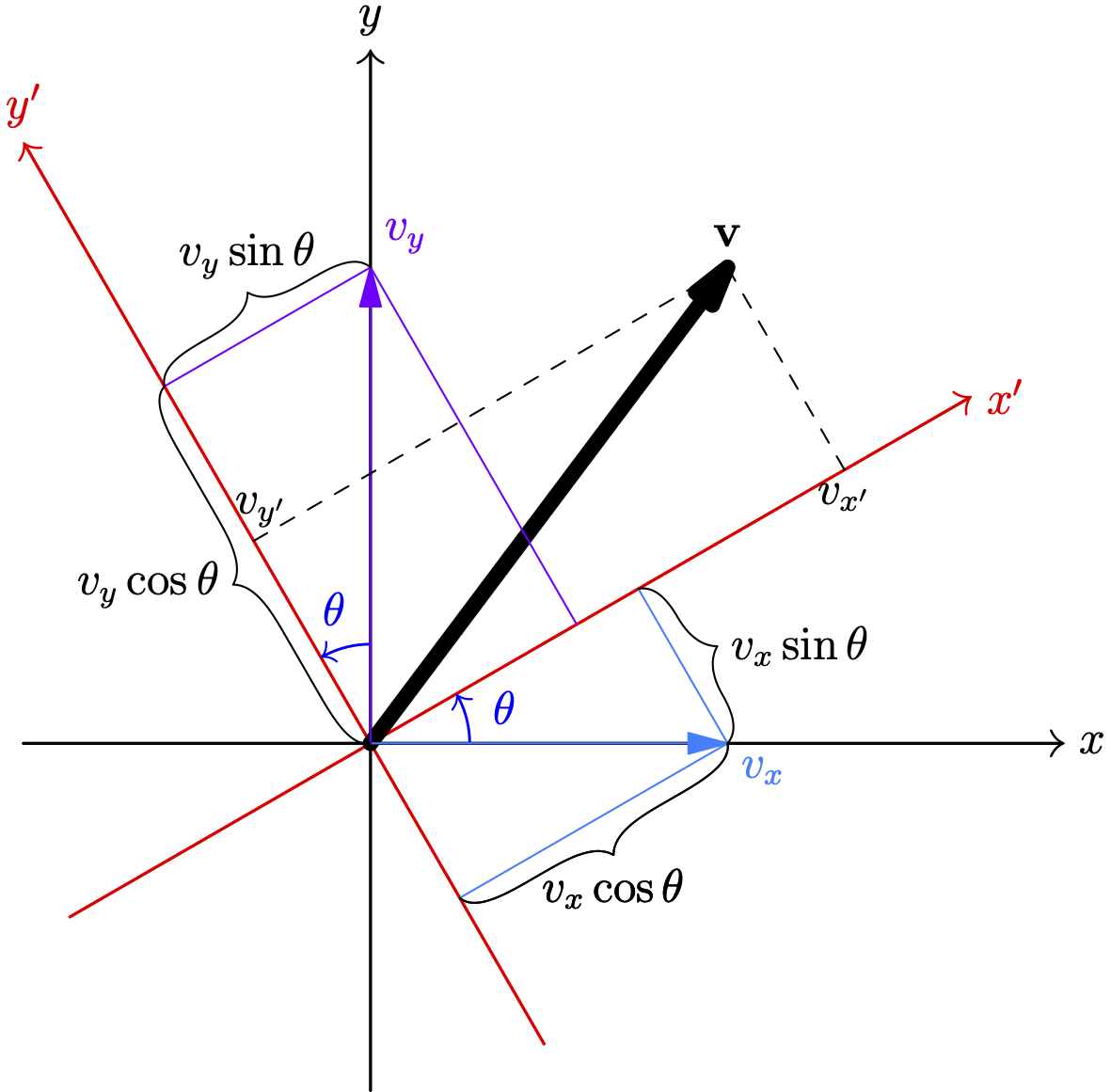
From the geometry (see the following figure), it is clear that we can write \[ \begin{aligned} v_{x'}=v_x\cos\theta+v_y \sin \theta\\ v_{y'}=v_y\cos\theta-v_x\sin \theta \end{aligned}\tag{1} \]

Using matrix notations, the above equations can be written as \[ \begin{bmatrix} v_{x'} & v_{y'} \end{bmatrix}=\begin{bmatrix} v_x & v_y \end{bmatrix}\begin{bmatrix} \cos \theta & -\sin\theta\\ \sin\theta & \cos\theta \end{bmatrix}\tag{2} \]

Second Approach

Suppose the unit vectors along the x- and y-axes be \(\mathbf{e}_1\) and \(\hat{\mathbf{e}}_2\) and the unit vectors along x’ and y-axes be \(\hat{\mathbf{e}}_{1'}\) and \(\hat{\mathbf{e}}_{2'}\). Let the components of a vector \(\mathbf{v}\) be \(v_x\) and \(v_y\) in the old system and \(v_{x'}\) and \(v_{y'}\) in the new system. Therefore, we have \[ v_x \hat{\mathbf{e}}_1+v_y \hat{\mathbf{e}}_2=v_{x'} \hat{\mathbf{e}}_{1'}+v_{y'} \hat{\mathbf{e}}_{2'}.\tag{3} \] If we express \(\hat{\mathbf{e}}_1\) and \(\hat{\mathbf{e}}_2\) in terms of \(\hat{\mathbf{e}}_{1'}\) and \(\hat{\mathbf{e}}_{2'}\), and substitute these expression into \(v_x \hat{\mathbf{e}}_1+v_y \hat{\mathbf{e}}_2\), we get an expression in the form of \(\alpha_1 \hat{\mathbf{e}}_{1'}+\alpha_2 \hat{\mathbf{e}}_{2'}\). Since the components of a vector with a basis is unique, we must have \(\alpha_1=v_{x'}\) and \(\alpha_2=v_{y'}\).

\[ \begin{aligned} \hat{\mathbf{e}}_1 &= l_{11'} \hat{\mathbf{e}}_{1'} + l_{12'} \hat{\mathbf{e}}_{2'}\\ \hat{\mathbf{e}}_2 &= l_{21'} \hat{\mathbf{e}}_{1'} + l_{22'}\hat{\mathbf{e}}_{2'} \end{aligned}\tag{4} \] which can be written as \[ \begin{bmatrix} \hat{\mathbf{e}}_1 \\ \hat{\mathbf{e}}_2 \end{bmatrix} = \begin{bmatrix} l_{11'} & l_{12'} \\ l_{21'} & l_{22'} \end{bmatrix} \begin{bmatrix} \hat{\mathbf{e}}_{1'} \\ \hat{\mathbf{e}}_{2'} \end{bmatrix}\tag{5} \]

We may write \(v_x \hat{\mathbf{e}}_1+v_y \hat{\mathbf{e}}_2\) as \[ v_x \hat{\mathbf{e}}_1+v_y \hat{\mathbf{e}}_2=\begin{bmatrix} v_x & v_y \end{bmatrix}\begin{bmatrix} \hat{\mathbf{e}}_1 \\ \hat{\mathbf{e}}_2 \end{bmatrix}\tag{6} \]

\[ \mathbf{v} = [v_x \;\; v_y] \begin{bmatrix} \hat{\mathbf{e}}_1 \\ \hat{\mathbf{e}}_2 \end{bmatrix} = [v_x \;\; v_y] \begin{bmatrix} l_{11'} & l_{12'} \\ l_{21'}' & l_{22'} \end{bmatrix} \begin{bmatrix} \hat{\mathbf{e}}_{1'} \\ \hat{\mathbf{e}}_{2'} \end{bmatrix}\tag{7} \]

By comparing the above equation with \[ \mathbf{v}=[v_{x'} \;\; v_{y'}] \begin{bmatrix} \hat{\mathbf{e}}_{1'} \\ \hat{\mathbf{e}}_{2'} \end{bmatrix} \] we realize, we must have \[ [v_{x'} \;\; v_{y'}] = [v_x \;\; v_y] \begin{bmatrix} l_{11'} & l_{12'} \\ l_{21'} & l_{22'} \end{bmatrix}\tag{8} \]

How can we determine \(l_{ij'}\)?

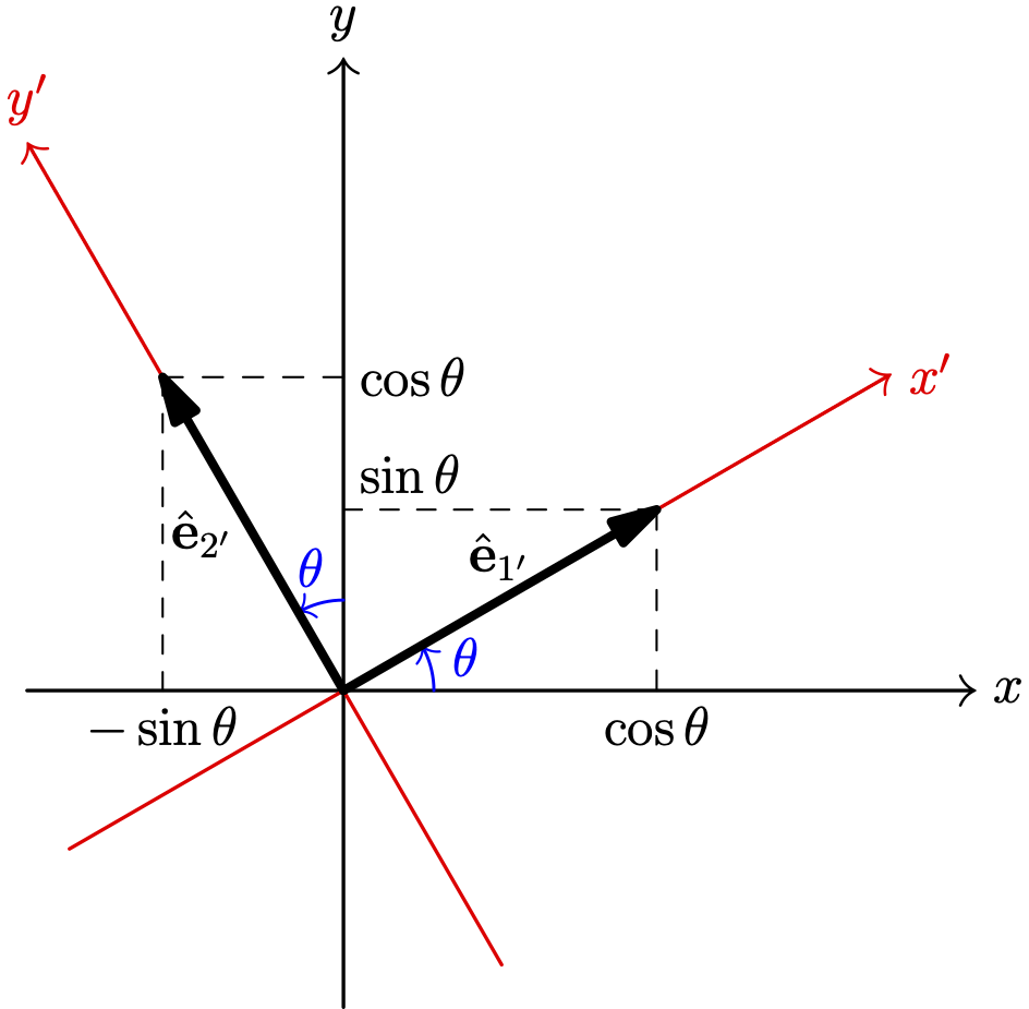
Let’s start with \[ \hat{\mathbf{e}}_1 = l_{11'} \hat{\mathbf{e}}_{1'} + l_{12'} \hat{\mathbf{e}}_{2'}. \] find the dot product of both sides by \(\hat{\mathbf{e}}_1\) \[ \begin{aligned} \hat{\mathbf{e}}_1 \cdot \hat{\mathbf{e}}_{1'}&= l_{11'} \underbrace{\hat{\mathbf{e}}_{1'} \cdot \hat{\mathbf{e}}_{1'}}_{1}+ l_{12'} \underbrace{\hat{\mathbf{e}}_{2'}\cdot \hat{\mathbf{e}}_{1'}}_0\\ &= l_{11'} \end{aligned} \] But the dot product of a two unit vector is equal to the cosine of the angle between them (which is the same as the cosine of the angle between x and x’). Also we notice that \(l_{11'}\) is the first component of \(\hat{\mathbf{e}}_{1'}\) in the old system \[ \hat{\mathbf{e}}_1 \cdot \hat{\mathbf{e}}_{1'} = l_{11'} = \cos(x, x') = \cos \theta = (\hat{\mathbf{e}}_1')_1 \] Similarly, we can show that \[ \hat{\mathbf{e}}_1 \cdot \hat{\mathbf{e}}_{2'} = l_{12'} = \cos(x, y') = \cos\!\left(\theta + \tfrac{\pi}{2}\right) = -\sin \theta = (\hat{\mathbf{e}}_{2'})_1 \] That is \(l_{12'}\) is the first component of \(\hat{\mathbf{e}}_{2'}\) in the old coordinate system. Similarly \[ \hat{\mathbf{e}}_2 \cdot \hat{\mathbf{e}}_1 = l_{21}' = \cos(y_1, x_1') = \cos\!\left(\theta - \tfrac{\pi}{2}\right) = \sin \theta = (\hat{\mathbf{e}}_1')_2 \] \[ \hat{\mathbf{e}}_2 \cdot \hat{\mathbf{e}}_2 = l_{22}' = \cos(y_1, y_1') = \cos \theta = (\hat{\mathbf{e}}_2')_2 \] Therefore, \[ \begin{bmatrix} l_{11'} & l_{12'} \\ l_{21'} & l_{22'} \end{bmatrix}=\begin{bmatrix} (\hat{\mathbf{e}}_{1'})_1 & (\hat{\mathbf{e}}_{2'})_1\\ (\hat{\mathbf{e}}_{1'})_2 & (\hat{\mathbf{e}}_{2'})_2 \end{bmatrix} \tag{9} \] That is, the columns of the above matrix are the unit vectors along the new coordinate system in the old coordinate system.

Since \(\hat{\mathbf{e}}_{1'}=[\cos \theta\ \ \ \sin\theta]\) and \(\hat{\mathbf{e}}_{2'}=[-\sin \theta\ \ \ \cos\theta]\), the matrix L is \[ L=\begin{bmatrix} \cos \theta & -\sin\theta\\ \sin\theta & \cos\theta \end{bmatrix}\tag{10} \] and we get \[ \begin{bmatrix} v_{x'} & v_{y'} \end{bmatrix}=\begin{bmatrix} v_x & v_y \end{bmatrix}\begin{bmatrix} \cos \theta & -\sin\theta\\ \sin\theta & \cos\theta \end{bmatrix}\tag{11} \] as before.

Transformation of a Vector in 3D

Now consider a more general case. Let the unit normal vectors along the new coordinate system be \(\hat{\mathbf{e}}_{1^\prime}\), \(\hat{\mathbf{e}}_{2^\prime}\), and \(\hat{\mathbf{e}}_{3^\prime}\). Let express the old unit normal vectors in terms of the new coordinate system: \[ \begin{aligned} \hat{\mathbf{e}}_1=l_{11'}\hat{\mathbf{e}}_{1^\prime}+l_{12'}\hat{\mathbf{e}}_{2^\prime}+l_{13'}\hat{\mathbf{e}}_{3^\prime}\\ \hat{\mathbf{e}}_2=l_{21'}\hat{\mathbf{e}}_{1^\prime}+l_{22'}\hat{\mathbf{e}}_{2^\prime}+l_{23'}\hat{\mathbf{e}}_{3^\prime}\\ \hat{\mathbf{e}}_3=l_{31'}\hat{\mathbf{e}}_{1^\prime}+l_{32'}\hat{\mathbf{e}}_{2^\prime}+l_{33'}\hat{\mathbf{e}}_{3^\prime} \end{aligned}\tag{12} \] You may wonder what \(l_{11'}\), \(l_{12'}\), … are. To determine \(l_{11'}\), let’s find the scalar product (a.k.a dot product) of \(\hat{\mathbf{e}}_1\) and \(\hat{\mathbf{e}}_1^\prime\): \[ \hat{\mathbf{e}}_1\cdot\hat{\mathbf{e}}_1^\prime=l_{11'}\hat{\mathbf{e}}_1^\prime\cdot\hat{\mathbf{e}}_1^\prime+l_{12'}\hat{\mathbf{e}}_2^\prime\cdot\hat{\mathbf{e}}_1^\prime+l_{13'}\hat{\mathbf{e}}_3^\prime\cdot\hat{\mathbf{e}}_1^\prime \] Since \(\hat{\mathbf{e}}_i^\prime\)’s are mutually perpendicular and the length of each is 1, then \[\hat{\mathbf{e}}_i^\prime\cdot\hat{\mathbf{e}}_j^\prime=\left\{\begin{aligned} &0 & \text{if } i\neq j\\ &1 & \text{if } i =j \end{aligned}\right.\tag{13} \] Therefore, \[ \hat{\mathbf{e}}_1\cdot\hat{\mathbf{e}}_1^\prime=l_{11'}\underbrace{\hat{\mathbf{e}}_1^\prime\cdot\hat{\mathbf{e}}_1^\prime}_{=1}+l_{12'}\underbrace{\hat{\mathbf{e}}_2^\prime\cdot\hat{\mathbf{e}}_1^\prime}_{=0}+l_{13'}\underbrace{\hat{\mathbf{e}}_3^\prime\cdot\hat{\mathbf{e}}_1^\prime}_{=0} \] \[ \begin{aligned} \Rightarrow l_{11'}&=\hat{\mathbf{e}}_1\cdot\hat{\mathbf{e}}_{1^\prime}\\ &=|\hat{\mathbf{e}}_1|\ |\hat{\mathbf{e}}_1^\prime|\cos(xx')\\ &=\cos(x,x') \end{aligned} \] because the angle between \(\hat{\mathbf{e}}_1\) and \(\hat{\mathbf{e}}_1^\prime\) is the same between \(x\)- and \(x'\)-axes. We also note that the \(l_{11'}\) is the first component of \(\hat{\mathbf{e}}_{1'}\) in the old system.

Similarly, \[ \hat{\mathbf{e}}_1\cdot\hat{\mathbf{e}}_2^\prime=l_{11'}\underbrace{\hat{\mathbf{e}}_1^\prime\cdot\hat{\mathbf{e}}_2^\prime}_{=0}+l_{12'}\underbrace{\hat{\mathbf{e}}_2^\prime\cdot\hat{\mathbf{e}}_2^\prime}_{=1}+l_{13'}\underbrace{\hat{\mathbf{e}}_3^\prime\cdot\hat{\mathbf{e}}_2^\prime}_{=0} \] \[ \begin{aligned} \Rightarrow l_{12'}&=\hat{\mathbf{e}}_1\cdot\hat{\mathbf{e}}_2^\prime\\ &=|\hat{\mathbf{e}}_1|\ |\hat{\mathbf{e}}_2^\prime|\cos(xy')\\ &=\cos(xy') \end{aligned} \] which is the same as the first component of \(\hat{\mathbf{e}}_{2'}\).

In general, we have \[ \begin{aligned} l_{ij'}&=\hat{\mathbf{e}}_i\cdot \hat{\mathbf{e}}_{j'}\\ &=\cos(x_i, x_{j^\prime})\\ &=\text{the }i\text{th coordinate of }\hat{\mathbf{e}}_j^\prime. \end{aligned}\tag{14} \]

Now we want to write the components of a vector \(\mathbf{v}\) in the new coordinate system. Let \(v_1\), \(v_2\), and \(v_3\) be the components of this vector in the old coordinate system. Therefore, \[ \mathbf{v}=v_1 \hat{\mathbf{e}}_1+v_2 \hat{\mathbf{e}}_2+v_3 \hat{\mathbf{e}}_3\tag{15} \] If we replace \(\hat{\mathbf{e}}_i\)’s in the above equation with the equations (ix), we obtain: \[ \begin{aligned} \mathbf{v}&=v_1 \hat{\mathbf{e}}_1+v_2 \hat{\mathbf{e}}_2+v_3 \hat{\mathbf{e}}_3\\ &=v_1(l_{11'}\hat{\mathbf{e}}_1^\prime+l_{12'}\hat{\mathbf{e}}_2^\prime+l_{13'}\hat{\mathbf{e}}_3^\prime)+v_2(l_{21'}\hat{\mathbf{e}}_1^\prime+l_{22'}\hat{\mathbf{e}}_2^\prime+l_{23'}\hat{\mathbf{e}}_3^\prime)\\ &\qquad +v_3(l_{31'}\hat{\mathbf{e}}_1^\prime+l_{32'}\hat{\mathbf{e}}_2^\prime+l_{33'}\hat{\mathbf{e}}_3^\prime)\\ &=(v_1l_{11'}+v_2l_{21'}+v_3l_{31'})\hat{\mathbf{e}}_1^\prime+(v_1 l_{12'}+v_2l_{22'}+v_3l_{32'})\hat{\mathbf{e}}_2^\prime\\ &\qquad +(v_1l_{13'}+v_2l_{23'}+v_3l_{33'})\hat{\mathbf{e}}_3^\prime \end{aligned}\tag{16} \] If in the new coordinate system, the components of \(\mathbf{v}\) are \(v_1^\prime\), \(v_2^\prime\), and \(v_3^\prime\), then we have \[ \mathbf{v}_{x'y'z'}=v_{1^\prime} \hat{\mathbf{e}}_{1^\prime}+v_{2^\prime} \hat{\mathbf{e}}_{2^\prime}+v_{3^\prime} \hat{\mathbf{e}}_{3^\prime}.\tag{17} \] By comparison of (16) and (17), we get \[ \begin{aligned} v_1^\prime&=v_1l_{11'}+v_2l_{21'}+v_3l_{31'}\\ v_2^\prime &= v_1 l_{12'}+v_2l_{22'}+v_3l_{32'}\\ v_3^\prime &=v_1l_{13'}+v_2l_{23'}+v_3l_{33'} \end{aligned}\tag{18} \] or concisely, \[ \begin{aligned} v_i^\prime&=v_1l_{1i'}+v_2l_{2i'}+v_3l_{3i'} \qquad (i=1,2,3)\\ &=\sum_{k=1}^3v_kl_{ki^\prime} \end{aligned}\tag{19} \] We may write (18) in the following matrix form: \[ \begin{aligned} \begin{bmatrix} v_{1^\prime} & v_{2^\prime} & v_{3^\prime} \end{bmatrix}&=\begin{bmatrix} v_1 & v_2 & v_3 \end{bmatrix} \begin{bmatrix} l_{11'} & l_{12'} & l_{13'}\\ l_{21'} &l_{22'} & l_{23'}\\ l_{31'} & l_{32'} & l_{33'} \end{bmatrix}\\[9pt] &=\begin{bmatrix} v_1 & v_2 & v_3 \end{bmatrix} \begin{bmatrix} | & | & |\\ \hat{\mathbf{e}}_1^\prime & \hat{\mathbf{e}}_2^\prime & \hat{\mathbf{e}}_3^\prime\\ | & | & | \end{bmatrix} \end{aligned}\tag{20} \] or \[ \mathbf{v}'=\mathbf{v}L.\tag{21} \]

Orthonormal Matrices

The matrix L has a special property: its inverse is the same as its transpose; that is \[ L^{-1}=L^T.\tag{22} \] Such matrices are called orthonormal matrices, as each column (and each row) form normal vectors that are mutually perpendicular.

Transformation of Stress

Now it’s time to study how we can express the components of stress in the new coordinate system in terms of its components in the old coordinate system.

Recall that to find the stress vector (or traction vector) \(\mathbf{t}\), we simply multiply the stress tensor \(\boldsymbol{\sigma}\) by the unit normal vector (\(\hat{\mathbf{n}}\)) of the desired plane; that is, \[ \mathbf{t}=\hat{\mathbf{n}}\boldsymbol{\sigma}\tag{23} \] Now if we change the coordinate system, we just learned, how to express the traction vector in the new system: \[ \mathbf{t}'=\mathbf{t}L=\underbrace{\hat{\mathbf{n}}\boldsymbol{\sigma}}_{\mathbf{t}}L\tag{24} \] However, when we are using the new coordinate system, the unit normal will be also expressed in this system. That is, we have to work with \(\hat{\mathbf{n}}'\) and not \(\hat{\mathbf{n}}\). ¹ However, \[ \hat{\mathbf{n}}'=\hat{\mathbf{n}}L. \] Multiplying both sides by the inverse of L (which is the same as its transpose because L is an orthonormal matrix) from the right, we get \[ \hat{\mathbf{n}}' L^T=\hat{\mathbf{n}}\underbrace{LL^T}_I=\hat{\mathbf{n}}.\tag{25} \] Now if we replace \(\hat{\mathbf{n}}\) in Equation (24) by (25), we get \[ \begin{aligned} \mathbf{t}'&=\hat{\mathbf{n}}\boldsymbol{\sigma}L\\ &=\underbrace{\hat{\mathbf{n}}' L^T}_{\hat{\mathbf{n}}} \boldsymbol{\sigma}L \end{aligned}\tag{26} \] The above equation shows that \(L^T\boldsymbol{\sigma}L\) is the same as the stress in the new coordinate system, as it gives the traction vector in the new system if we multiply the unit normal of any desired plane in the new system. Therefore, \[ \boxed{\boldsymbol{\sigma}^\prime=L^T\boldsymbol{\sigma} L.}\tag{27} \] where L is a matrix whose columns are the components of unit vectors in the old coordinate system.

Now let’s see the formula for a 2D problem where the x- and y-axes are rotated by \(\theta\). In this case: \[ \hat{\mathbf{e}}_1^\prime = \begin{bmatrix} \cos\theta & \sin\theta \end{bmatrix} \qquad \hat{\mathbf{e}}_2^\prime = \begin{bmatrix} -\sin\theta & \cos\theta \end{bmatrix} \] Therefore, \[ L=\begin{bmatrix} \cos\theta & -\sin\theta\\ \sin\theta & \cos\theta \end{bmatrix}\tag{28} \] and \[ \begin{bmatrix} \sigma_{x'} & \tau_{x'y'}\\ \tau_{y'x'} & \sigma_{y'} \end{bmatrix}=\begin{bmatrix} \cos \theta & \sin\theta\\ -\sin\theta & \cos\theta \end{bmatrix}\begin{bmatrix} \sigma_{x} & \tau_{xy}\\ \tau_{yx} & \sigma_{y} \end{bmatrix}\begin{bmatrix} \cos \theta & -\sin\theta\\ \sin\theta & \cos\theta \end{bmatrix}\tag{29} \]

It follows from the above equations that \[ \begin{aligned} \sigma_{x^\prime} & =\sigma_x \cos ^2 \theta+\sigma_y \sin ^2 \theta+2 \tau_{x y} \sin \theta \cos \theta \\ \sigma_{y^\prime} & =\sigma_{x} \sin ^2 \theta+\sigma_y \cos ^2 \theta-2 \tau_{x y} \sin \theta \cos \theta \\ \tau_{x^\prime y^\prime} & =\left(-\sigma_x+\sigma_y\right) \sin \theta \cos \theta+\tau_{x y}\left(\cos ^2 \theta-\sin ^2 \theta\right)\end{aligned}\tag{30} \] which are the same equations we obtained previously.

Appendix: Vector Expansion in Orthonormal Basis

Suppose \(\hat{\mathbf{E}}_1, \hat{\mathbf{E}}_2, \hat{\mathbf{E}}_3\) are unit vectors that are mutually perpendicular.
Any vector in \(\mathbb{R}^3\) can be written as: \[ \mathbf{v} = v_1 \hat{\mathbf{E}}_1 + v_2 \hat{\mathbf{E}}_2 + v_3 \hat{\mathbf{E}}_3 \] To find \(v_1\), take the dot product with \(\hat{\mathbf{E}}_1\): \[ \mathbf{v} \cdot \hat{\mathbf{E}}_1 = v_1 (\hat{\mathbf{E}}_1 \cdot \hat{\mathbf{E}}_1) + v_2 (\hat{\mathbf{E}}_2 \cdot \hat{\mathbf{E}}_1) + v_3 (\hat{\mathbf{E}}_3 \cdot \hat{\mathbf{E}}_1) \] Since the basis is orthonormal: \[ \mathbf{v} \cdot \hat{\mathbf{E}}_1 = v_1 (1) + v_2 (0) + v_3 (0) \] \[ \Rightarrow v_1 = \mathbf{v} \cdot \hat{\mathbf{E}}_1 \] Similarly:

\[ v_2 = \mathbf{v} \cdot \hat{\mathbf{E}}_2, \quad v_3 = \mathbf{v} \cdot \hat{\mathbf{E}}_3 \]