Resistance Strain Gage1
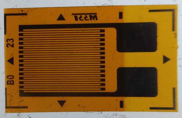
Except in a few cases involving contact stresses, it is not possible to measure stress directly. Therefore, experimental measurements of stress are actually based on measured strains and are converted to stresses by means of Hooke’s law and the more general relationships which are given in the next chapter. The most universal strain-measuring device is the bonded-wire resistance gage, frequently called the SR-4 strain gage. These gages are made up of several loops of fine wire or foil of special composition, which are cemented to the surface of the body to be studied. If the cement is considerably stronger than the gauge itself, the gauge effectively becomes an integral part of the body. As a result, when the body is subjected to strain along the direction of the gauge, the wire within the gauge and the body will undergo the same strain, and their electrical resistance is altered. The change in resistance, which is proportional to strain, can be accurately determined with a simple Wheatstone-bridge circuit. The high sensitivity, stability, comparative ruggedness, and ease of application make resistance strain gages a very powerful tool for strain determination.
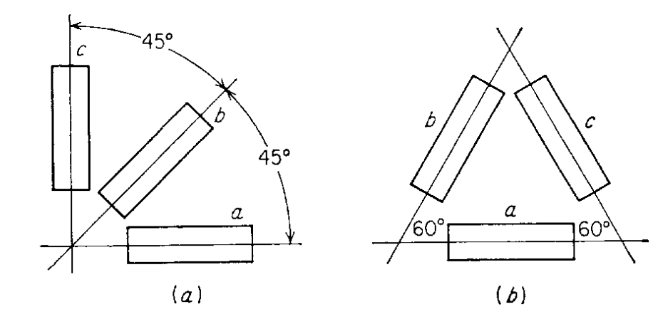
For practical problems of experimental stress analysis it is often important to determine the principal stresses. If the principal directions are known, gages can be oriented in these directions and the principal stresses determined quite readily. In the general case the direction of the principal strains will not be known, so that it will be necessary to determine the orientation and magnitude of the principal strains from the measured strains in arbitrary directions. Because no stress can act perpendicular to a free surface, strain-gage measurements involve a two-dimensional state of strain. The state of strain is completely determined if ϵxx, ϵyy, and γxy can be measured. However, strain gages can make only direct readings of linear strain, while shear strains must be determined indirectly. Therefore, it is the usual practice to use three strain gages separated at fixed angles in the form of a “rosette,” as in the following figure. Strain-gage readings at three values of θ will give three simultaneous equations, which can be solved for ϵxx, ϵyy, and γxy. Then we can determine the principal strains.
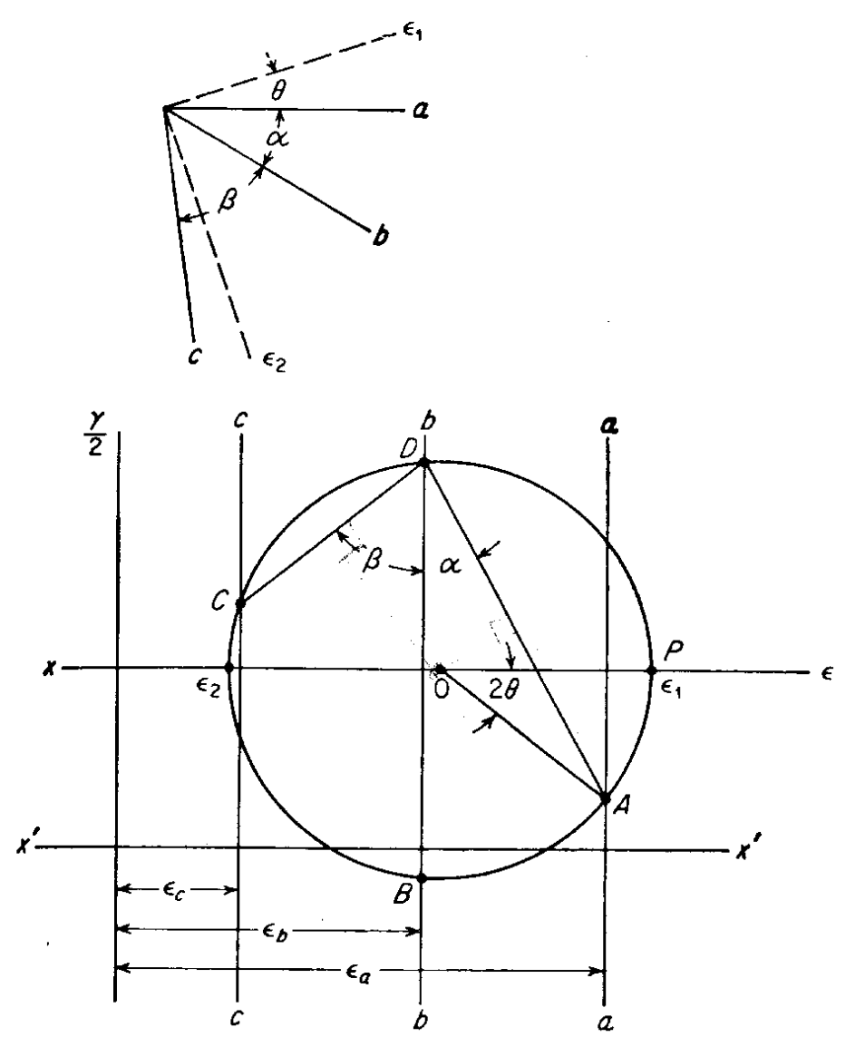
A more convenient method of determining a principal strains from strain-gage readings than the solution of three simultaneous equations in three unknowns is the use of Mohr’s circle. In constructing a Mohr’s circle representation of strain, values of linear normal strain ϵ are plotted along the x-axis, and the shear strain γ divided by 2 (or ϵxy) is plotted along the y axis. The following figure shows the Mohr’s circle construction for the generalized strain-gage rosette illustrated at the top of the figure. Strain-gage readings ϵa, ϵb, and ϵc for normal strains are available for three gages situated at arbitrary angles α and β. The objective is to determine the magnitude and orientation of the principal strains ϵ1 and ϵ2.
- Along an arbitrary axis X’X’ lay off vertical lines aa, bb, and cc corresponding to the strains ϵa, ϵb, and ϵc.
- From any point on the line bb (middle strain gage) draw a line DA at an angle α with bb and intersecting aa at point A. In the same way, lay off DC intersecting cc at point C.
- Construct a circle through A, C, and D. The center of this circle is at O, determined by the intersection of the perpendicular bisectors to CD and AD.
- Points A, B, and C on the circle give the values of ϵ and γ/2 (measured from the new x axis through O) for the three gages.
- Values of the principal strains are determined by the intersection of the circle with the new x axis through O. The angular relationship of ϵ1 to the gage a is one-half the angle AOP on the Mohr’s circle (AOP = 2θ).
A 60° (delta) strain rosette at a point on a free surface yields the following measurements: ε(0°) = 100 μ, ε(60°) = - 200 μ, and ε(120°) = 300 μ. Determine (a) the in-plane principal strains (ε₁ and ε₂) and (b) the true maximum shear strain (γmax).
Solution
Recall that: \[ \epsilon_{x^\prime}=\frac{\epsilon_x+\epsilon_y}{2}+\frac{\epsilon_x-\epsilon_y}{2} \cos 2 \theta+\epsilon_{x y} \sin 2 \theta \] Now in this equation, once we put \(\theta=0\) and \(\epsilon_{x'}=100\) μ and get one equation. Once we put \(\theta=60^\circ\) and \(\epsilon_{x'}=\) 200 μ for the second equation and put \(\theta=120^\circ\) and \(\epsilon_{x'}=\) -300 μ for the third equation.
\[ 100\ \mu = \frac{\epsilon_x+\epsilon_y}{2}+\frac{\epsilon_x-\epsilon_y}{2}=\epsilon_x. \] \[ \begin{aligned} 200\ \mu &=\frac{\epsilon_x+\epsilon_y}{2}+\frac{\epsilon_x-\epsilon_y}{2} \overbrace{\cos (120^\circ)}^{-1/2}+\epsilon_{x y}\, \overbrace{\sin (120^\circ)}^{\sqrt{3}/2}\\ &=\frac{1}{4}\epsilon_x+\frac{3}{4}\epsilon_y+\frac{\sqrt{3}}{2}\epsilon_{xy} \end{aligned} \] \[ \begin{aligned} -300\ \mu &=\frac{\epsilon_x+\epsilon_y}{2}+\frac{\epsilon_x-\epsilon_y}{2} \overbrace{\cos (240^\circ)}^{-1/2}+\epsilon_{x y}\, \overbrace{\sin (240^\circ)}^{-\sqrt{3}/2}\\ &=\frac{1}{4}\epsilon_x+\frac{3}{4}\epsilon_y-\frac{\sqrt{3}}{2}\epsilon_{xy} \end{aligned} \] Solving this system of three equations gives: \[ \epsilon_x=100\ \mu, \quad \epsilon_y=33.33\ \mu, \quad \epsilon_{xy}=-288.675\ \mu. \] The strain tensor at this point is therefore: \[ \boldsymbol{\epsilon}=\begin{bmatrix} 100 & -288.675\\ -288.675& 33.33 \end{bmatrix}\mu \] The principal strains (ε₁ and ε₂) are the eigenvalues of the strain tensor. The eigenvalues of this matrix are \[ \epsilon_1=107.0378\ \mu,\qquad \epsilon_2=-373.7034\ \mu. \] These are the maximum and minimum in-plane normal strains. Another way of calculating them is through the following formula: \[ \epsilon_{1,2}=\frac{\epsilon_x+\epsilon_y}{2}\pm \sqrt{\left(\frac{\epsilon_1-\epsilon_2}{2}\right)^2+\epsilon_{xy}^2} \] Using the above formula, we get the same result.
The maximum shear strain is \[ \gamma_{\max}=|2\epsilon_{\max}|=\epsilon_1-\epsilon_2=480.74 \]
Digital Image Correlation (DIC)
Another method for measuring surface strain, especially in micro- and nano-scale mechanical testing, is Digital Image Correlation (DIC). This non-contact optical method utilizes digital cameras to track the movement of a speckle pattern applied to the surface of an object. By comparing images of the object before and during deformation, DIC software can calculate the displacement and strain over the entire surface.
Of course. Here are concise descriptions for each patterning method at different scales.
Macroscale Patterning Methods
- Spray Paint: A fine mist of paint (e.g., matte black) is sprayed over a contrasting base coat (e.g., matte white) to create a random pattern of droplets suitable for general-purpose DIC.
- Markers and Stamps: A random dot pattern is applied manually with markers for quick tests or transferred consistently using a pre-fabricated random stamp.
Microscale Patterning Methods
- Nanoparticle Deposition: Nanoparticles suspended in a solvent are airbrushed or dropped onto a surface; the solvent evaporates to leave a fine, random speckle pattern ideal for Scanning Electric Microscopy (SEM) analysis.
- Photolithography: A light-sensitive coating is exposed to UV light through a random-pattern mask to create a very precise and durable speckle pattern.
- E-Beam Lithography: A focused beam of electrons writes an ultra-high-resolution random pattern onto a sensitive surface layer, offering excellent control over feature size.
- Focused Ion Beam (FIB) Milling: A high-energy ion beam physically etches a random pattern directly into the specimen’s surface, ensuring perfect adhesion as the pattern is part of the material itself.
- Inherent Microstructure: The material’s own natural features, such as metallic grain boundaries or different phases, are used as the pattern, eliminating the need for any artificial application.
Nanoscale Patterning Methods
- Self-Assembled Nanoparticles: Nanoparticles or quantum dots are chemically induced to arrange themselves into a random monolayer, creating a dense pattern suitable for nanoscale imaging.
- Atomic/Crystalline Structure: At the highest magnifications, the material’s own atomic lattice is imaged and used as the pattern, allowing for the direct measurement of strain at the crystal level.
The basic principle of DIC involves capturing a reference image of the speckled surface in an undeformed state. As the body deforms, a series of images is taken. The DIC software then divides the reference image into smaller subsets (facets) and tracks the movement of these subsets in the subsequent images of the deformed body by analyzing the unique grayscale pattern within each one. This tracking provides a map of displacements, from which strain fields can be calculated.
For two-dimensional strain analysis, a single camera can be used. However, for complex surfaces or to measure out-of-plane displacement, a stereo-DIC setup with two cameras is employed to provide three-dimensional measurements.
At macroscale strain gages may offer higher accuracy for very small strains (e.g., less than 300 microstrain), DIC provides a powerful and comprehensive tool for understanding the full-field mechanical behavior of materials and structures.
- From George E. Dieter, Mechanical Metallugry (1961), 1st edition, McGraw-Hill.↩︎