The concepts now assembled enable us to explain some of the major meanings assigned to the word “random” in the mathematical theory of probability.
One meaning arises in connection with the notion of a random sample of a random variable . Let us consider a random variable \(X\) , of which it is possible to make repeated measurements, denoted by \(X_{1}, X_{2}, \ldots, X_{n}, \ldots\) For example, \(X_{1}, X_{2}, \ldots, X_{n}\) may be the lifetimes of each of \(n\) electric light bulbs, or they may be the numbers on balls drawn (with or without replacement) from an urn containing balls numbered 1 to 100, and so on. The set of \(n\) measurements \(X_{1}, X_{2}, \ldots, X_{n}\) is spoken of as a sample of size \(n\) of the random variable \(X\) , by which is meant that each of the measurements \(X_{k}\) , for \(k=1,2, \ldots, n\) , is a random variable whose distribution function \(F_{X_{k}}(\cdot)\) is equal, as a function of \(x\) , to the distribution function \(F_{X}(\cdot)\) of the random variable \(X\) . If, further, the random variables \(X_{1}, X_{2}, \ldots, X_{n}\) are independent, then we say that \(X_{1}, X_{2}, \ldots, X_{n}\) is a random sample (or an independent sample) of size \(n\) of the random variable \(X\) . Thus the adjective “random,” when used to describe a sample of a random variable, indicates that the members of the sample are independent identically distributed random variables.
Example 7A . Suppose that the life in hours of electronic tubes of a certain type is known to be approximately normally distributed with parameters \(m=160\) and \(\sigma=20\) . What is the probability that a random sample of four tubes will contain no tube with a lifetime of less than 180 hours?
Solution
Let \(X_{1}, X_{2}, X_{3}\) , and \(X_{4}\) denote the respective lifetimes of the four tubes in the sample. The assumption that the tubes constitute a random sample of a random variable normally distributed with parameters \(m=160\) and \(\sigma=20\) is to be interpreted as assuming that the random variables \(X_{1}, X_{2}, X_{3}\) , and \(X_{4}\) are independent, with individual probability density functions, for \(k=1, \ldots, 4\) ,
\[f_{X_{k}}(x)=\frac{1}{20 \sqrt{2 \pi}} \exp \left[-\frac{1}{2}\left(\frac{x-160}{20}\right)^{2}\right]. \tag{7.1}\]
The probability that each tube in the sample has a lifetime greater than, or equal to, 180 hours, is given by
\begin{align} & P\left[X_{1} \geq 180, X_{2} \geq 180, X_{3} \geq 180, X_{4} \geq 180\right] \\ & \quad=P\left[X_{1} \geq 180\right] P\left[X_{2} \geq 180\right] P\left[X_{3} \geq 180\right] P\left[X_{4} \geq 180\right]=(0.159)^{4}, \end{align}
since \(P\left[X_{k} \geq 180\right]=1-\Phi\left(\frac{180-160}{20}\right)=1-\Phi(1)=0.1587\) .
A second meaning of the word “random” arises when it is used to describe a sample drawn from a finite population. A sample, each of whose components is drawn from a finite population, is said to be a random sample if at each draw all candidates available for selection have an equal probability of being selected. The word “random” was used in this sense throughout Chapter 2 .
Example 7B . As in example 7A, consider electronic tubes of a certain type whose lifetimes are normally distributed with parameters \(m=160\) and \(\sigma=20\) . Let a random sample of four tubes be put into a box. Choose a tube at random from the box. What is the probability that the tube selected will have a lifetime greater than 180 hours?
Solution
For \(k=0,1, \ldots, 4\) let \(A_{k}\) be the event that the box contains \(k\) tubes with a lifetime greater than 180 hours. Since the tube lifetimes are independent random variables with probability density functions given by (7.1), it follows that \[P\left[A_{k}\right]=\left(\begin{array}{l} 4 \tag{7.2}\\ k \end{array}\right)(0.1587)^{k}(0.8413)^{4-k}.\] Let \(B\) be the event that the tube selected from the box has a lifetime greater than 180 hours. The assumption that the tube is selected at random is to be interpreted as assuming that
\[P\left[B \mid A_{k}\right]=\frac{k}{4}, \quad k=0,1, \ldots, 4. \tag{7.3}\]
The probability of the event \(B\) is then given by
\[P[B]=\sum_{k=0}^{4} P\left[B \mid A_{k}\right] P\left[A_{k}\right]=\sum_{k=1}^{4} \frac{k}{4}\left(\begin{array}{l} 4 \tag{7.4}\\ k \end{array}\right) p^{k} q^{4-k},\]
where we have let \(p=0.1587, q=0.8413\) . Then
\[P[B]=p \sum_{k=1}^{4}\left(\begin{array}{c} 3 \tag{7.5}\\ k-1 \end{array}\right) p^{k-1} q^{3-(k-1)}=p,\]
so that the probability that a tube selected at random from a random sample will have a lifetime greater than 180 hours is the same as the probability that any tube of the type under consideration will have a lifetime greater than 180 hours. A similar result was obtained in example 4D of Chapter 3. A theorem generalizing and unifying these results is given in theoretical exercise 4.1 of Chapter 4.
The word random has a third meaning, which is frequently encountered. The phrase “a point randomly chosen from the interval \(a\) to \(b\) ” is used for brevity to describe a random variable obeying a uniform probability law over the interval \(a\) to \(b\) , whereas the phrase “ \(n\) points chosen randomly from the interval \(a\) to \(b\) ” is used for brevity to describe \(n\) independent random variables obeying uniform probability laws over the interval \(a\) to \(b\) . Problems involving randomly chosen points have long been discussed by probabilists under the heading of “geometrical probabilities”. In modern terminology problems involving geometrical probabilities may be formulated as problems involving independent random variables, each obeying a uniform probability law.
Example 7C . Two points are selected randomly on a line of length \(a\) so as to be on opposite sides of the mid-point of the line. Find the probability that the distance between them is less than \(\frac{1}{3}a\) .
Solution
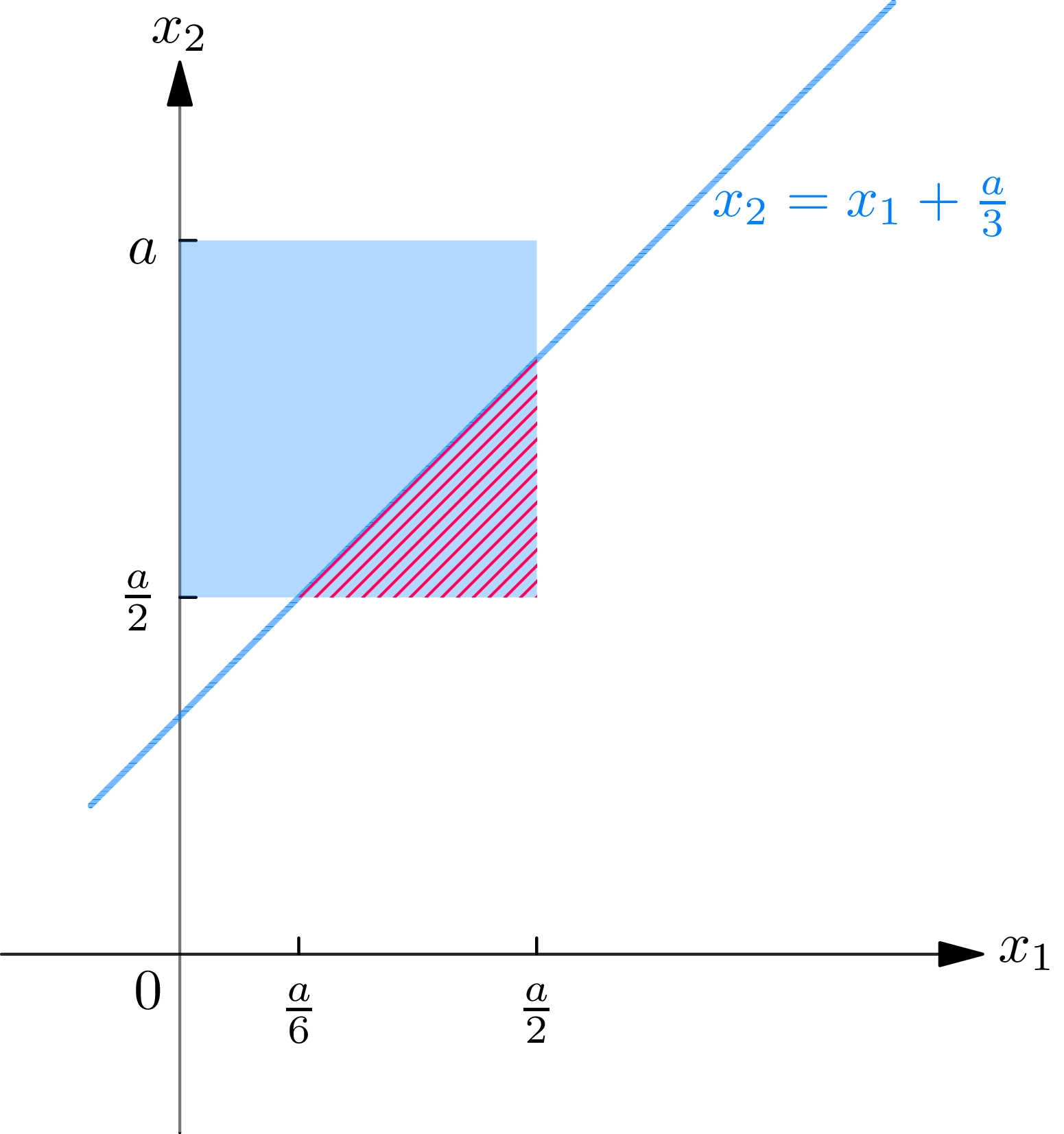
Introduce a coordinate system on the line so that its left-hand endpoint is 0 and its right-hand endpoint is \(a\) . Let \(X_{1}\) be the coordinate of the point selected randomly in the interval 0 to \(\frac{1}{2} a\) , and let \(X_{2}\) be the coordinate of the point selected randomly in the interval \(\frac{1}{2} a\) to \(a\) . We assume that the random variables \(X_{1}\) and \(X_{2}\) are independent and that each obeys a uniform probability law over its interval. The joint probability density function of \(X_{1}\) and \(X_{2}\) is then \[f_{X_{1}, X_{2}}\left(x_{1}, x_{2}\right) =\left\{ \begin{aligned} &\frac{4}{a^{2}}, && \text{for } 0 < x_{1} < \frac{a}{2}, \quad \frac{a}{2} < x_{2} < a \\ &0, && \text{otherwise.} \end{aligned}\right. \tag{7.6}\] The event \(B\) that the distance between the two points selected is less than \(\frac{1}{3} a\) is then the event \(\left[X_{2}-X_{1}<\frac{1}{3} a\right]\) . The probability of this event is the probability attached to the hatched area in Fig. 7A. However, this probability can be represented as the ratio of the area of the cross-hatched triangle and the area of the shaded rectangle; thus \[P\left[X_{2}-X_{1}<\frac{1}{3} a\right]=\frac{1 / 2[(1 / 3) a]^{2}}{[(1 / 2) a]^{2}}=\frac{2}{9}. \tag{7.7}\]
Example 7D . Consider again the random variables \(X_{1}\) and \(X_{2}\) defined in example 7C. Find the probability that the three line segments (from 0 to \(X_{1}\) , from \(X_{1}\) to \(X_{2}\) , and from \(X_{2}\) to \(a\) ) could be made to form the three sides of a triangle.
Solution
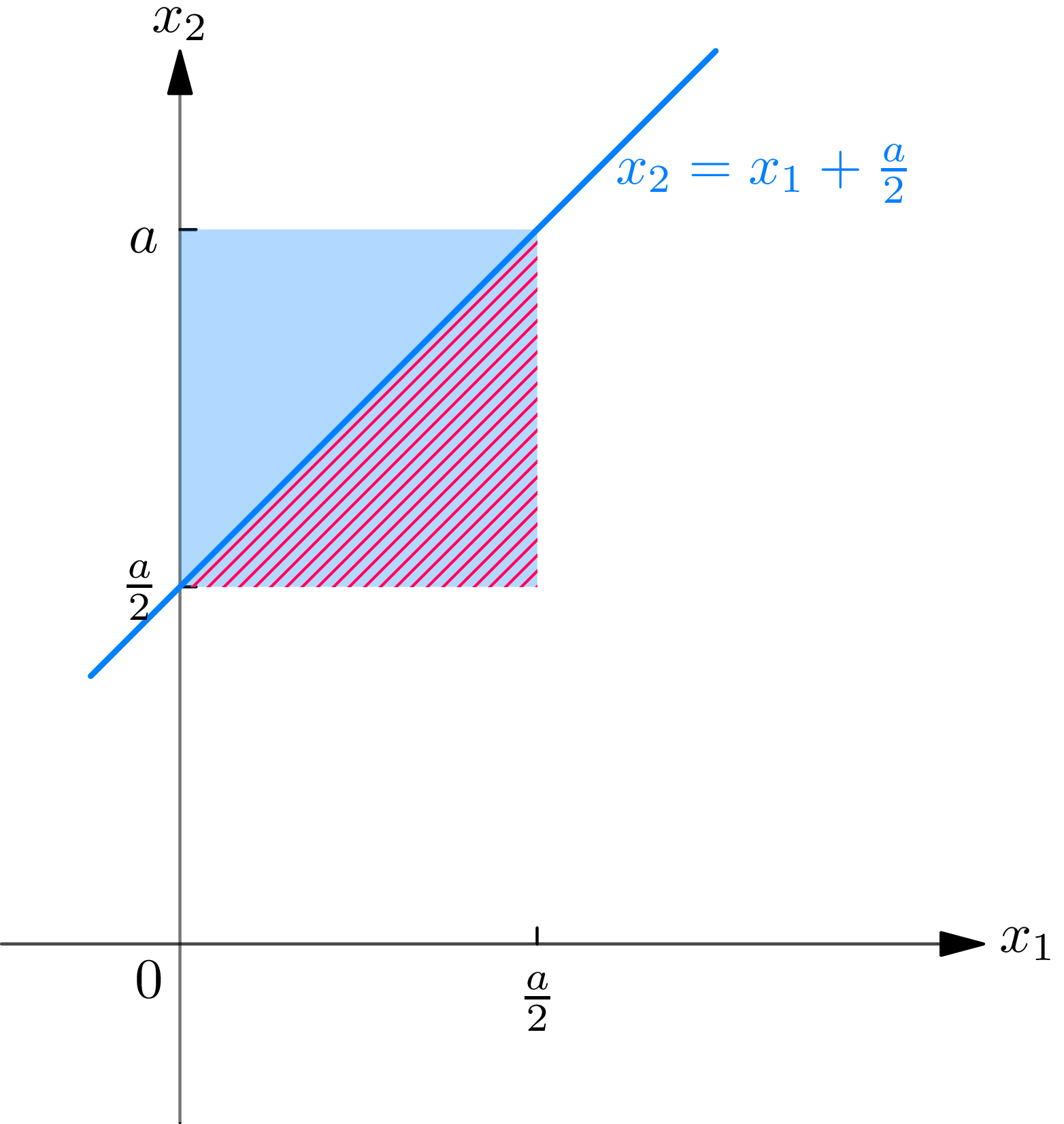
In order that the three-line segments mentioned can form a triangle, it is necessary and sufficient that the following inequalities be fulfilled (why?): \[\begin{array}{lll} X_{1}<\left(X_{2}-X_{1}\right)+\left(a-X_{2}\right) & \text { or } & 2 X_{1}The probability of these inequalities being fulfilled is the probability of the hatched area in Fig. 7B, which is clearly \(\frac{1}{2}\) . It might be noted that if each of the two points, with coordinates \(X_{1}\) and \(X_{2}\) , are chosen randomly on the interval 0 to \(a\) , then the probability is only \(\frac{1}{4}\) that the three line segments determined by the two points could be made to form the three sides of a triangle.
Problems involving geometrical probability have played a major role in the development of the modern conception of probability. In the nineteenth century the Laplacean definition of probability was widely accepted. It was thought that probability problems could be given unique solutions by means of finding the proper framework of “equally likely” descriptions. To contradict this point of view, examples were constructed that admitted of several equally plausible, but incompatible, solutions. We now discuss an example similar to one given by Joseph Bertrand in his treatise Calcul des probabilités , Paris, 1889, p. 4, and later called by Poincaré, “Bertrand’s paradox”. It was pointed out to the author by one of his students that this example should serve as a warning to all persons who adopt practical
policies on the basis of theoretical solutions, without first establishing that the assumptions underlying the solutions are in accord with the experimentally observed facts.
Example 7E . Bertrand’s paradox . Let a chord be chosen randomly in a circle of radius \(r\) . What is the probability that the length \(X\) of the chord will be less than the radius \(r\)?
Solution
It is not clear what is meant by a randomly chosen chord. In order to give meaning to this phrase, we shall reformulate the problem as one involving randomly chosen points. We shall state two methods for randomly choosing points to determine a chord. In this manner we obtain two distinct answers for the probability \(P[X
One method is as follows: let \(Y_{1}\) and \(Y_{2}\) be points chosen randomly in the interval 0 to \(2 \pi\) and the interval 0 to \(r\) , respectively. Draw a chord by letting \(Y_{1}\) be the angle made by the chord with a fixed reference line and by letting \(Y_{2}\) be the (perpendicular) distance of the mid-point of the chord from the center of the circle (see Fig. 7C). A second method of randomly choosing a chord is as follows: let \(Z_{1}\) and \(Z_{2}\) be points chosen randomly in the interval 0 to \(2 \pi\) and the interval 0 to \(\pi / 2\) , respectively. Draw a chord by letting \(Z_{1}\) and \(Z_{2}\) be the angles indicated in Fig. 7D. The reader may be able to think of other methods of choosing points to determine a chord. Six different solutions of Bertrand’s paradox are given in Czuber, Wahrscheinlichkeitsrechnung , B. G. Teubner, Leipzig, 1908, pp. 106–109.
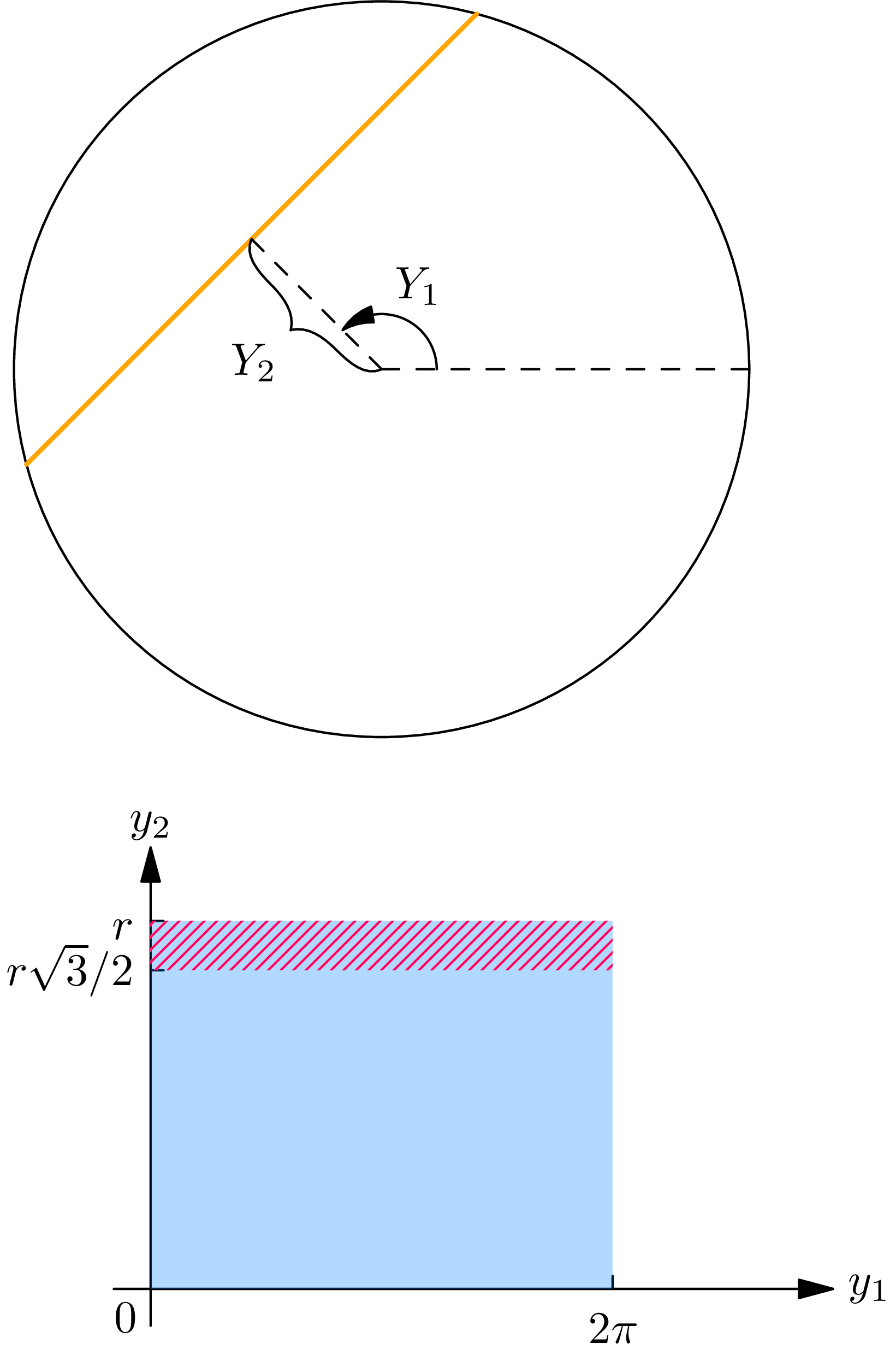
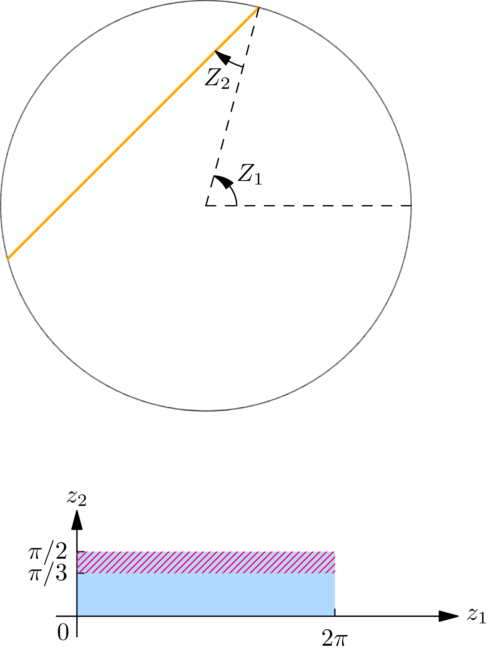
The length \(X\) of the chord may be expressed in terms of the random variables \(Y_{1}, Y_{2}, Z_{1}\) , and \(Z_{2}\) : \[X=2 \sqrt{r^{2}-Y_{2}^{2}} \quad \text { or } \quad X=2 r \cos Z_{2}. \tag{7.9}\] Consequently \(P[X
It should be noted that random experiments could be performed in such a way that either (7.10) or (7.11) would be the correct probability in the sense of the frequency definition of probability. If a disk of diameter \(2 r\) were cut out of cardboard and thrown at random on a table ruled with parallel lines a distance \(2 r\) apart, then one and only one of these lines would cross the disk. All distances from the center would be equally likely, and (7.10) would represent the probability that the chord drawn by the line across the disk would have a length less than \(r\) . On the other hand, if the disk were held by a pivot through a point on its edge, which point lay upon a certain straight line, and spun randomly about this point, then (7.11) would represent the probability that the chord drawn by the line across the disk would have a length less than \(r\) .
The following example has many important extensions and practical applications.
Example 7F . The probability of an uncrowded road . Along a straight road, \(L\) miles long, are \(n\) distinguishable persons, distributed at random. Show that the probability that no two persons will be less than a distance \(d\) miles apart is equal to, for \(d\) such that \((n-1) d \leq L\) ,
\[\left(1-(n-1) \frac{d}{L}\right)^{n}. \tag{7.12}\]
Solution
For \(j=1,2, \ldots, n\) let \(X_{j}\) denote the position of the \(j\) th person. We assume that \(X_{1}, X_{2}, \ldots, X_{n}\) are independent random variables, each uniformly distributed over the interval 0 to \(L\) . Their joint probability density function is then given by
\begin{align} f_{X_{1}, X_{2}, \ldots, X_{n}}\left(x_{1}, x_{2}, \ldots, x_{n}\right) = \begin{cases} \frac{1}{L^{n}}, & \text{if } 0 \leq x_{1}, x_{2}, \ldots, x_{n} \leq L \\ 0, & \text{otherwise.} \end{cases} \tag{7.13} \end{align}
Next, for each permutation, or ordered \(n\) -tuple chosen without replacement, \(\left(i_{1}, i_{2}, \ldots, i_{n}\right)\) of the integers 1 to \(n\) , define
\[I\left(i_{1}, i_{2}, \ldots, i_{n}\right)=\left\{\left(x_{1}, x_{2}, \ldots, x_{n}\right): \quad x_{i_{1}}
Thus \(I\left(i_{1}, i_{2}, \ldots, i_{n}\right)\) is a zone of points in \(n\) -dimensional Euclidean space. There are \(n\) ! such zones that are mutually exclusive. The union of all zones does not include all the points in \(n\) -dimensional space, since an \(n\) -tuple \(\left(x_{1}, x_{2}, \ldots, x_{n}\right)\) that contains two equal components does not lie in any zone. However, we are able to ignore the set of points not included in any of the zones, since this set has probability zero under a continuous probability law. Now the event \(B\) that no two persons are less than a distance \(d\) apart may be represented as the set of \(n\) -tuples \(\left(x_{1}, x_{2}, \ldots, x_{n}\right)\) for which the distance \(\left|x_{i}-x_{j}\right|\) between any two components is greater than \(d\) . To find the probability of \(B\) , we must first find the probability of the intersection of \(B\) and each zone \(I\left(i_{1}, i_{2}, \ldots, i_{n}\right)\) . We may represent this intersection as follows:
\begin{align} B I\left(i_{1}, i_{2}, \ldots, i_{n}\right)=\left\{\left(x_{1}, x_{2}, \ldots, x_{n}\right): \quad 0
Consequently,
\begin{align} & P_{X_{1}, X_{2}, \ldots, X_{n}}\left[B I\left(i_{1}, i_{2}, \ldots, i_{n}\right)\right] \tag{7.16}\\ &=\frac{1}{L^{n}} \int_{0}^{L-(n-1) d} d x_{i_{1}} \int_{x_{i_{1}}+d}^{L-(n-2) d} d x_{i_{2}} \cdots \int_{x_{i_{n-1}}+d}^{L} d x_{i_{n}} \\ &=\int_{0}^{1-(n-1) d^{\prime}} d u_{1} \int_{u_{1}+d^{\prime}}^{1-(n-2) d^{\prime}} d u_{2} \cdots \int_{u_{n-2}+d^{\prime}}^{1-d^{\prime}} d u_{n-1} \int_{u_{n-1}+d^{\prime}}^{1} d u_{n}, \end{align}
in which we have made the change of variables \(u_{1}=x_{i_{1}} / L, \ldots, u_{n}=\) \(x_{i_{n}} / L\) , and have set \(d^{\prime}=d / L\) . The last written integral is readily evaluated and is seen to be equal to, for \(k=2, \ldots, n-1\) ,
\begin{align} \int_{0}^{1-(n-1) d^{\prime}} d u_{1} & \int_{u_{1}+d^{\prime}}^{1-(n-2) d^{\prime}} d u_{2} \cdots \int_{u_{k-1}+d^{\prime}}^{1-(n-k) d^{\prime}} d u_{k} \\ & \times \frac{1}{(n-k) !}\left(1-(n-k) d^{\prime}-u_{k}\right)^{n-k}. \end{align}
The probability of \(B\) is equal to the product of \(n\) ! and the probability of the intersection of \(B\) and any zone \(I\left(i_{1}, i_{2}, \ldots, i_{n}\right)\) . The proof of (7.12) is now complete.
In a similar manner one may solve the following problem.
Example 7G . Packing cylinders randomly on a rod . Consider a horizontal rod of length \(L\) on which \(n\) equal cylinders, each of length \(c\) , are distributed at random. The probability that no two cylinders will be less than \(d\) apart is equal to, for \(d\) such that \(L \geq n c+(n-1)d\) ,
\[\left(1-\frac{(n-1) d}{L-nc}\right)^{n}. \tag{7.18}\]
The foregoing considerations, together with (6.2) of Chapter 2, establish an extremely useful result.
The Random Division of an Interval or a Circle . Suppose that a straight line of length \(L\) is divided into \(n\) sub-intervals by \((n-1)\) points chosen at random on the line or that a circle of circumference \(L\) is divided into \(n\) sub-intervals by \(n\) points chosen at random on the circle. Then the probability \(P_{k}\) that exactly \(k\) of the sub-intervals will exceed \(d\) in length is given by
\[P_{k}=\left(\begin{array}{l} n \tag{7.19}\\ k \end{array}\right) \sum_{j=k}^{[L / d]}(-1)^{j-k}\left(\begin{array}{c} n-k \\ n-j \end{array}\right)\left(1-\frac{j d}{L}\right)^{n-1}.\]
It may clarify the meaning of (7.19) to express it in terms of random variables. Let \(X_{1}, X_{2}, \ldots, X_{n-1}\) be the coordinates of the \(n-1\) points chosen randomly on the line (a similar discussion may be given for the circle.) Then \(X_{1}, X_{2}, \ldots, X_{n-1}\) are independent random variables, each uniformly distributed on the interval 0 to \(L\) . Define new random variables \(Y_{1}, Y_{2}, \ldots, Y_{n-1}: \quad Y_{1}\) is equal to the minimum of \(X_{1}, X_{2}, \ldots, X_{n-1}\) ; \(Y_{2}\) is equal to the second smallest number among \(X_{1}, X_{2}, \ldots, X_{n-1}\) ; and, so on, up to \(Y_{n-1}\) , which is equal to the maximum of \(X_{1}, X_{2}, \ldots, X_{n-1}\) . The random variables \(Y_{1}, Y_{2}, \ldots, Y_{n-1}\) thus constitute a reordering of the random variables \(X_{1}, X_{2}, \ldots, X_{n-1}\) , according to increasing magnitude. For this reason, the random variables \(Y_{1}, Y_{1}, \ldots, Y_{n-1}\) are called the order statistics corresponding to \(X_{1}, X_{2}, \ldots, X_{n-1}\) . The random variable \(Y_{k}\) , for \(k=1,2, \ldots, n-1\) , is usually spoken of as the \(k\) th smallest value among \(X_{1}, X_{2}, \ldots, X_{n-1}\) .
The lengths \(W_{1}, W_{2}, \ldots, W_{n}\) of the \(n\) successive subintervals into which the \((n-1)\) randomly chosen points divide the line may now be expressed:
\begin{align} W_{1} = Y_{1}, \quad W_{2}= Y_{2} - Y_{1}, \ldots, \quad\quad W_{j} & = Y_{j} - Y_{j-1}, \ldots, \\ W_{n} & = L - Y_{n-1}. \tag{7.20} \end{align}
The probability \(P_{k}\) is the probability that exactly \(k\) of the \(n\) events \(\left[W_{1}>d\right],\left[W_{2}>d\right], \ldots,\left[W_{n}>d\right]\) will occur. To prove (7.19), one needs only to verify that for any integer \(j\) the probability that \(j\) specified subintervals will exceed \(d\) in length is equal to
\[\left(1-\frac{j d}{L}\right)^{n-1} \quad \text { if } 0 \leq j \leq L / d. \tag{7.21}\]
References to the large variety of problems to which (7.19) is applicable may be found in two papers: J. O. Irwin, “A Unified Derivation of Some Well-known Frequency Distributions of Interest in Biometry and Statistics,” Journal of the Royal Statistical Society A , Vol. 118 (1955), pp. 389398, and L. Takacs, “On a general probability theorem and its application in the theory of stochastic processes”, Proceedings of the Cambridge Philosophical Society, Vol. 54 (1958), pp. 219–224.
Theoretical Exercises
7.1 . Buffon’s Needle Problem . A smooth table is ruled with equidistant parallel lines at distance \(D\) apart. A needle of length \(L
7.2 . A straight line of unit length is divided into \(n\) subintervals by \(n-1\) points chosen at random. For \(r=1,2, \ldots, n-1\) , show that the probability that none of \(r\) specified subintervals will be less than \(d\) in length is equal to \[(1-r d)^{n-1} \tag{7.22}\] Hence, using (6.3) of Chapter 2, conclude that the probability that at least 1 of the \(n\) subintervals will exceed \(d\) in length is equal to \begin{align} n(1-d)^{n-1}-& \left(\begin{array}{l} n \\ 2 \end{array}\right)(1-2 d)^{n-1} \tag{7.23}\\ &+\cdots(-1)^{r-1}\left(\begin{array}{l} n \\ r \end{array}\right)(1-r d)^{n-1}+\cdots, \end{align} the series continuing as long as the terms \((1-r d)^{n-1}, r=1,2, \ldots\) are positive.
Exercises
7.1 . A young man and a young lady plan to meet between 5 and 6 P.M., each agreeing not to wait more than 10 minutes for the other. Find the probability that they will meet if they arrive independently at random times between 5 and 6 P.M.
Answer
\(\frac{1}{3} \frac{1}{10}\) .
7.2 . Consider light bulbs produced by a machine for which it is known that the life \(X\) in hours of a light bulb produced by the machine is a random variable with probability density function
\begin{align} f_{X}(x) & = \begin{cases} \dfrac{1}{1000} e^{-(x / 1000)}, & \text{for } x > 0 \\ 0, & \text{otherwise.} \end{cases} \end{align}
Consider a box containing 100 such bulbs, selected randomly from the output of the machine.
(i) What is the probability that a bulb selected randomly from the box will have a lifetime greater than 1020 hours?
(ii) What is the probability that a sample of 5 bulbs selected randomly from the box will contain (a) at least 1 bulb, (b) 4 or more bulbs with a lifetime greater than 1020 hours?
(iii) Find approximately the probability that the box will contain between 30 and 40 bulbs, inclusive, with a lifetime greater than 1020 hours.
7.3 . Six soldiers take up random positions on a road 2 miles long. What is the probability that the distance between any two soldiers will be more than (i) \(\frac{1}{2}\) , (ii) \(\frac{1}{3}\) , (iii) \(\frac{1}{4}\) of a mile?
Answer
(i) 0; (ii) \(\left(\frac{1}{6}\right)^{6}\) ; (iii) \(\left(\frac{3}{8}\right)^{6}\) .
7.4 . Another version of Bertrand’s paradox . Let a chord be drawn at random in a given circle. What is the probability that the length of the chord will be greater than the side of the equilateral triangle inscribed in that circle?
7.5 . A point is chosen randomly on each of 2 adjacent sides of a square. Find the probability that the area of the triangle formed by the sides of the square and the line joining the 2 points will be (i) less than \(\frac{1}{8}\) of the area of the square, (ii) greater than \(\frac{1}{2}\) of the area of the square.
Answer
(i) \(\frac{1}{4}(1+\ln 4)\) ; (ii) 0.
7.6 . Three points are chosen randomly on the circumference of a circle. What is the probability that there will be a semicircle in which all will lie?
7.7 . A line is divided into 3 subintervals by choosing 2 points randomly on the line. Find the probability that the 3-line segments thus formed could be made to form the sides of a triangle.
Answer
\(\frac{1}{4}\) .
7.8 . Find the probability that the roots of the equation \(x^{2}+2 X_{1} x+X_{2}=0\) will be real if (i) \(X_{1}\) and \(X_{2}\) are randomly chosen between 0 and 1, (ii) \(X_{1}\) is randomly chosen between 0 and 1, and \(X_{2}\) is randomly chosen between -1 and 1.
7.9 . In the interval \(0\) to \(1\) , \(n\) points are chosen randomly. Find (i) the probability that the point lying farthest to the right will be to the right of the number 0.6, (ii) the probability that the point lying farthest to the left will be to the left of the number 0.6, (iii) the probability that the point lying next farthest to the left will be to the right of the number 0.6.
Answer
(i) \(1-(0.6)^{n}\) ; (ii) \(1-(0.4)^{n}\) ; (iii) \((0.4)^{n}+n(0.6)(0.4)^{n-1}\) .
7.10 . A straight line of unit length is divided into 10 subintervals by 9 points chosen at random. For any (i) number \(d>\frac{1}{2}\) , (ii) number \(d>\frac{1}{3}\) find the probability that none of the subintervals will exceed \(d\) in length.