Chain Rule

16.1 INTRODUCTION
16.2 LECTURE
- 16.2.1 The Multivariable Chain Rule
- 16.2.2 Scalar Functions and the Gradient
16.3 EXAMPLES
16.4 ILLUSTRATIONS

16.1 INTRODUCTION

16.1.1 Building Complex Functions from Basic Ones

In calculus, we can build from basic functions more general functions. One possibility is to add functions like $f (x) + g (x) = x^{2} + \sin (x)$ . An other possibility is to multiply functions like $f (x) g (x) = x^{2} \sin (x)$ . A third possibility is to combine functions like $f \circ g (x) = f (g (x)) = \sin^{2} (x)$ . The composition of functions is non-commutative: $f \circ g \neq g \circ f$ . Indeed, we have $g \circ f (x) = \sin (x^{2})$ which is completely different from $f \circ g (x) = \sin^{2} (x)$ .

Illustration for Chain Rule — **Figure 1.** $f : ℝ^{p} \to ℝ^{n}$ and $g : ℝ^{m} \to ℝ^{p}$ can be combined to $f (g) : ℝ^{m} \to ℝ^{n}$ .

16.1.2 The Chain Rule: From Single Variable to Higher Dimensions

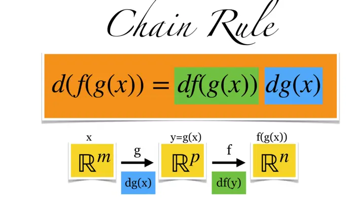
How can we express the rate of change of a composite function in terms of the basic functions it is built of? For the sum of two functions, we have the addition rule (f+g)^{\prime}(x)=f^{\prime}(x)+g^{\prime}(x), for multiplication we have the product rule (f g)^{\prime}(x)=f^{\prime}(x) g(x)+f(x) g(x). We usually just write (f+g)^{\prime}=f^{\prime}+g^{\prime} or (f g)^{\prime}=f^{\prime} g+f g^{\prime} and do not always write the argument. As you know from single variable calculus, the derivative of the composite function is given by chain rule. This is (f \circ g)^{\prime}=f^{\prime}(g) g^{\prime}. Written out in more details with argument, we can write \frac{d}{d x} f(g(x))=\frac{d}{d x} f^{\prime}(g(x)) g^{\prime}(x). We generalize this here to higher dimensions. Instead of $\frac{d}{d x} f$ we just write $d f$ . This is the Jacobean matrix we know. Now, the same rule holds as before $d f (g (x)) = d f (g (x)) d g (x)$ and this is called the chain rule in higher dimensions. On the right hand side, we have the matrix product of two matrices.

16.1.3 Dimensions and the Chain Rule

Let us see why this makes sense in terms of dimensions: $g : ℝ^{m} \to ℝ^{p}$ and $f :$ $ℝ^{p} \to ℝ^{n}$ , then $d g (x) \in M (p, m)$ and $d f (g (x)) \in M (n, p)$ and $d f (g (x)) d g (x) \in M (n, m)$ which is the same type of matrix than $d (f \circ g)$ because $f \circ g (x)$ maps $ℝ^{m} \to ℝ^{n}$ so that also $d (f \circ g) (x) \in M (n, m)$ . The name chain rule comes because it deals with functions that are chained together.

16.2 LECTURE

16.2.1 The Multivariable Chain Rule

Given a differentiable function $r : ℝ^{m} \to ℝ^{p}$ , its derivative at $x$ is the Jacobian matrix $d r (x) \in M (p, m)$ . If $f : ℝ^{p} \to ℝ^{n}$ is another function with $d f (y) \in M (n, p)$ , we can combine them and form $f \circ r (x) = f (r (x)) : ℝ^{m} \to ℝ^{n}$ . The matrices $d f (y) \in$ $M (n, p)$ and $d r (x) \in M (p, m)$ combine to the matrix product $d f d r$ at a point. This matrix is in $M (n, m)$ . The multi-variable chain rule is:

Theorem 1. $d (f \circ r) (x) = d f (r (x)) d r (x)$ .

16.2.2 Scalar Functions and the Gradient

For $m = n = p = 1$ , the single variable calculus case, we have d f(x)=f^{\prime}(x) and (f \circ r)^{\prime}(x)=f^{\prime}(r(x)) r^{\prime}(x). In general, $d f$ is now a matrix rather than a number. By checking a single matrix entry, we reduce to the case $n = m = 1$ . In that case, $f : ℝ^{p} \to ℝ$ is a scalar function. While $d f$ is a row vector, we define the column vector $\nabla f = d f^{T} = [f_{x_{1}}, f_{x_{2}}, \dots f_{x_{p}}]^{T} .$ If $r : ℝ \to ℝ^{p}$ is a curve, we write r^{\prime}(t)= [x_{1}^{\prime}(t), \cdots, x_{p}^{\prime}(t)]^{T} instead of $d r (t)$ . The symbol $\nabla$ is addressed also as "nabla".¹ The special case $n = m = 1$ is:

Theorem 2. \frac{d}{d t} f(r(t))=\nabla f(r(t)) \cdot r^{\prime}(t).

Proof. $\frac{d}{d t} f (x_{1} (t), x_{2} (t), \dots, x_{p} (t))$ is the limit $h \to 0$ of \begin{aligned} & \big[f\big(x_{1}(t+h), x_{2}(t+h), \ldots, x_{p}(t+h)\big)-f\big(x_{1}(t), x_{2}(t), \ldots, x_{p}(t)\big)\big] / h \\ = & \big[f\big(x_{1}(t+h), x_{2}(t+h), \ldots, x_{p}(t+h)\big)-f\big(x_{1}(t), x_{2}(t+h), \ldots, x_{p}(t+h)\big)\big] / h \\ + & \big[f\big(x_{1}(t), x_{2}(t+h), \ldots, x_{p}(t+h)\big)-f\big(x_{1}(t), x_{2}(t), \ldots, x_{p}(t+h)\big)\big] / h+\cdots \\ + & \big[f\big(x_{1}(t), x_{2}(t), \ldots, x_{p}(t+h)\big)-f\big(x_{1}(t), x_{2}(t), \ldots, x_{p}(t)\big)\big] / h \end{aligned} which is ( $1$ D chain rule) in the limit $h \to 0$ the sum f_{x_{1}}(x) x_{1}^{\prime}(t)+\cdots+f_{x_{p}}(x) x_{p}^{\prime}(t).

Proof of the general case: Let $h = f \circ r$ . The entry $i j$ of the Jacobian matrix $d h (x)$ is $d h_{i j} (x) = \partial_{x_{j}} h_{i} (x) = \partial_{x_{j}} f_{i} (r (x))$ . The case of the entry $i j$ reduces with $t = x_{j}$ and $h_{i} = f$ to the case when $r (t)$ is a curve and $f (x)$ is a scalar function. This is the case we have proven already. ◻

16.3 EXAMPLES

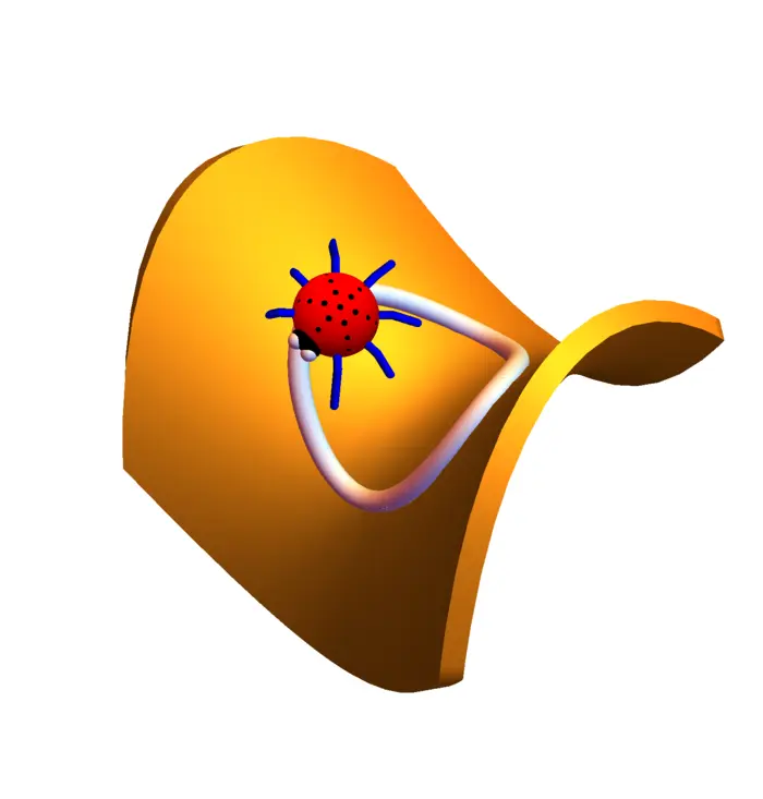
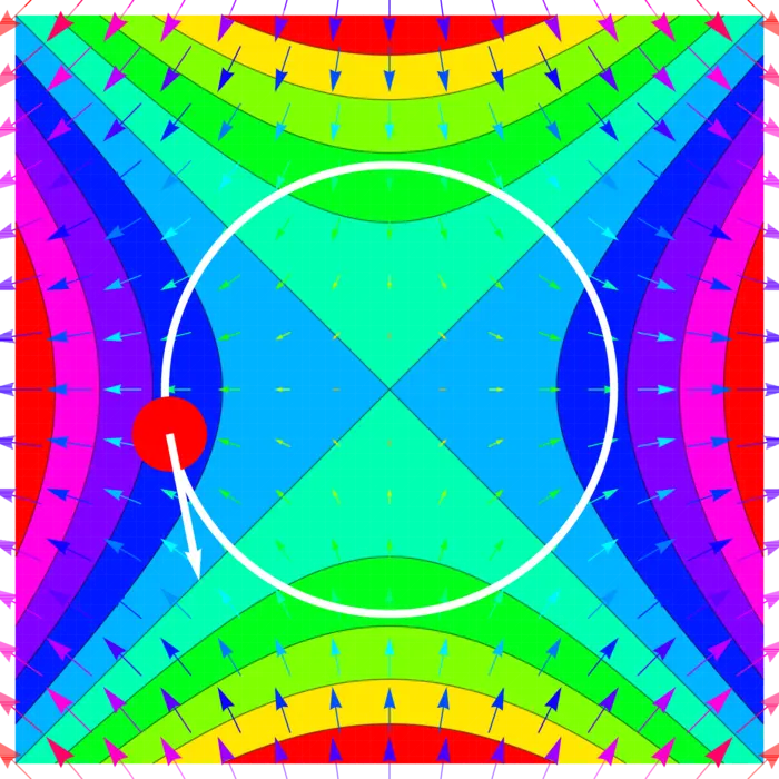
Example 1. Assume a ladybug walks on a circle $r (t) = [\begin{matrix} \cos (t) \\ \sin (t) \end{matrix}]$ and $f (x, y) = x^{2} - y^{2}$ is the temperature at the position $(x, y)$ , then $f (r (t))$ is the rate of change of the temperature. We can write $f (r (t)) = \cos^{2} (t) - \sin^{2} (t) = \cos (2 t) .$ Now, $d / d t f (r (t)) = - 2 \sin (2 t)$ . The gradient of $f$ and the velocity are \nabla f(x, y)=\left[\begin{array}{r}2 x \\ -2 y\end{array}\right], \quad r^{\prime}(t)=\left[\begin{array}{r}-\sin (t) \\ \cos (t)\end{array}\right]. Now \begin{aligned} \nabla f(r(t)) \cdot r^{\prime}(t)&=\left[\begin{array}{r} 2 \cos (t) \\ -2 \sin (t) \end{array}\right] \cdot\left[\begin{array}{r} -\sin (t) \\ \cos (t) \end{array}\right]\\ &=-4 \cos (t) \sin (t)\\ &=-2 \sin (2 t). \end{aligned}

16.4 ILLUSTRATIONS

16.4.1 Power from Potential: A Chain Rule Connection

The case $n = m = 1$ is extremely important. The chain rule $d / d t f (r (t)) =$ \nabla f(r(t)) \cdot r^{\prime}(t) tells that the rate of change of the potential energy $f (r (t))$ at the position $r (t)$ is the dot product of the force $F = \nabla f (r (t))$ at the point and the velocity with which we move. The right hand side is power $=$ force times velocity. We will use this later in the fundamental theorem of line integrals.

16.4.2 Chaos via Derivatives: Lyapunov Exponents and Entropy in Iterated Maps

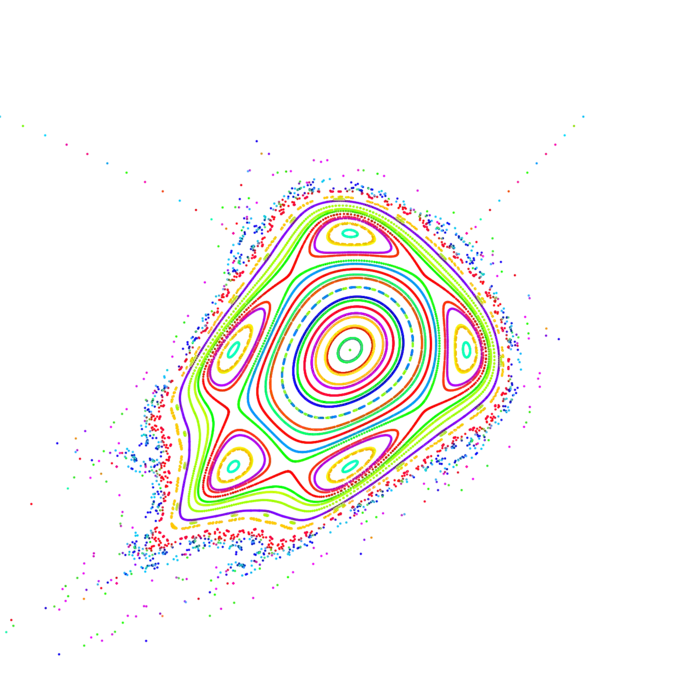
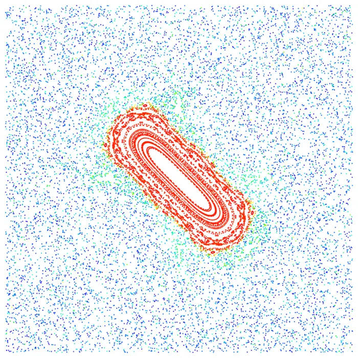
If $f, g : ℝ^{m} \to ℝ^{m}$ , then $f \circ g$ is again a map from $ℝ^{m}$ to $ℝ^{n}$ . We can also iterate a map like $x \to f (x) \to f (f (x)) \to f (f (f (x))) \dots$ The derivative $d f^{n} (x)$ is by the chain rule the product $d f (f^{n - 1} (x)) \dots d f (f (x)) d f (x)$ of Jacobian matrices. The number $λ (x) = \underset{n \to \infty}{lim sup} (1 / n) \log (| d f^{n} (x) |)$ is called the Lyapunov exponent of the map $f$ at the point $x$ . It measures the amount of chaos, the "sensitive dependence on initial conditions" of $f$ . These numbers are hard to estimate mathematically. Already for simple examples like the Chirikov map $f ([x, y]) = [2 x - y + c \sin (x), x],$ one can measure positive entropy $S (c)$ . A conjecture of Sinai tells that that the entropy of the map is positive for large $c$ . Measurements show that this entropy $S (c) = \int_{0}^{2 π} \int_{0}^{2 π} λ (x, y) d x d y / (4 π^{2})$ satisfies $S (x) \geq \log (c / 2)$ . The conjecture is still open.²

16.4.3 Hamilton’s Equations and Energy Conservation

If $H (x, y)$ is a function called the Hamiltonian and x^{\prime}(t)=H_{y}(x, y), y^{\prime}(t)= $- H_{x} (x, y)$ , then $d / d t H (x (t), y (t)) = 0$ . This can be interpreted as energy conservation. We see that a Hamiltonian differential equation always preserves the energy. For the pendulum, $H (x, y) = y^{2} / 2 - \cos (x)$ , we have x^{\prime}=y, y^{\prime}=-\sin (x) or x^{\prime \prime}=-\sin (x).

16.4.4 The Chain Rule Unlocks Inverses

The chain rule is useful to get derivatives of inverse functions. Like \begin{aligned} 1=\frac{d}{d x} x&=\frac{d}{d x} \sin (\arcsin (x))\\ &=\cos (\arcsin (x)) \arcsin ^{\prime}(x) \end{aligned} which then gives \begin{aligned} \arcsin ^{\prime}(x)&=1 / \sqrt{1-\sin ^{2}(\arcsin (x))}\\ &=1 / \sqrt{1-x^{2}}. \end{aligned}

16.4.5 Implicit Differentiation: Finding the Mystery Slope

Assume $f (x, y) = x^{3} y + x^{5} y^{4} - 2 - \sin (x - y) = 0$ is a curve. We can not solve for $y$ . Still, we can assume $f (x, y (x)) = 0$ . Differentiation using the chain rule gives f_{x}(x, y(x))+f_{y}(x, y(x)) y^{\prime}(x)=0. Therefore y^{\prime}(x)=-\frac{f_{x}(x, y(x))}{f_{y}(x, y(x))} In the above example, the point $(x, y) = (1, 1)$ is on the curve. Now $g_{x} (x, y) =$ $3 + 5 - 1 = 7$ and $g_{y} (x, y) = 1 + 4 + 1 = 6$ . So, g^{\prime}(1)=-7 / 6. This is called implicit differentiation. We could compute with it the derivative of a function which was not known.

16.4.6 Guaranteed Solutions: The Implicit Function Theorem

The implicit function theorem assures that a differentiable implicit function $g (x)$ exists near a root $(a, b)$ of a differentiable function $f (x, y)$ .

Theorem 3. If $f (a, b) = 0$ , $f_{y} (a, b) \neq 0$ there exists $c > 0$ and a function $g \in C^{1} ([b - c, b + c])$ with $f (x, g (x)) = 0$ .

Proof. Let $c$ be so small that for fixed $x \in [a - c, a + c]$ , the function $y \in [b - c, b + c] \to h (y) = f (x, y)$ has the property $h (b - c) < 0$ and $h (b + c) > 0$ and h^{\prime}(y) \neq 0 in $[b - c, b + c]$ . The intermediate value theorem for $h$ now assures a unique root $z = g (x)$ of $h$ near $b$ . The chain rule formula above then assures that for $a - c < x < a + c$ , the differential quotient $[g (x + h) - g (x)] / h$ written down for $g$ has a limit $- f_{x} (x, g (x)) / f_{y} (x, g (x))$ . ◻

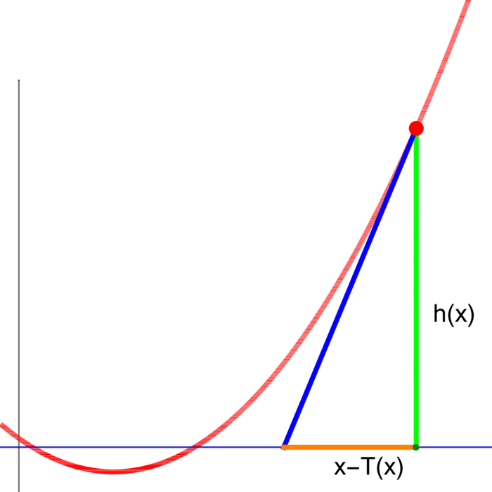
P.S. We can get the root of $h$ by applying Newton steps T(y)=y-h(y) / h^{\prime}(y). Taylor (seen in the next class) shows the error is squared in every step. The Newton step $T (y) = y - d h (y)^{- 1} h (y)$ works also in arbitrary dimensions. One can prove the implicit function theorem by just establishing that Id $- T = d h^{- 1} h$ is a contraction and then use the Banach fixed point theorem to get a fixed point of $Id - T$ which is a root of $h$ .

Units 16 and 17 are together taught on Wednesday. Homework is all in unit 17.

Etymology tells that the symbol is inspired by a Egyptian or Phoenician harp.↩︎
To generate orbits, see http://www.math.harvard.edu/k̃nill/technology/chirikov/.↩︎

Table of Contents