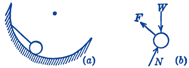
In many cases the particle under consideration will not be completely free, but will be constrained by various connections to move in a certain way. For example, the particle might be a bead sliding along a wire, in which case the geometrical constraint would be that the particle is required to follow the wire. In another case the particle might be required to remain on a particular surface, as in Fig. 1a. In all such cases the behavior of the constraint is to introduce a reactive force into the problem which enforces the constraint.

In Fig. 1b is shown the free-body diagram of the particle. The active forces in this case have been assumed to be the weight in the case of a frictionless contact. Such a normal constraint, corresponding to frictionless surfaces in contact, is called an ideal constraint, and we shall limit our discussion, in the following pages, to such ideal constraints.

In the case of a constrained particle, it will be necessary to alter somewhat our definition of a virtual displacement, since it is clear that certain displacements, such as those normal to a constraining surface, will not be possible. In such a case the virtual displacement cannot be any arbitrary displacement, but must be restricted to those displacements which are permitted by the constraints. We thus define a virtual displacement as an infinitesimal displacement of the particle which is compatible with the constraints. The word “virtual” therefore acquires the significance of the word “possible,” in that it represents all of those infinitesimal displacements which are consistent with the geometry of the system. It will be seen that this more general definition of a virtual displacement includes the definition given for a free particle as a special case.

The equation expressing the principle of virtual displacements can now be written as follows, where we have separated the forces into two types, the active forces \(\mathbf{F}\) and the ideal reactive forces \(\mathbf{F}_{r}\) : \[ \sum\left[\left(F_{x}+F_{x r}\right) \delta x+\left(F_{y}+F_{y r}\right) \delta y+\left(F_{z}+F_{z r}\right) \delta z\right]=0 \]

This equation will still represent the conditions of equilibrium under our new definition of a virtual displacement. In the case of a constraining surface, for example, such virtual displacements would lie in a plane tangent to the surface. Our equation would then prohibit any resultant force in that plane, while the constraint itself insures that the forces normal to the plane balance out.

We next write the above equation in the following form: \[ \sum\left(F_{x} \delta x+F_{y} \delta y+F_{z} \delta z\right)+\sum\left(F_{x r} \delta x+F_{y r} \delta y+F_{z r} \delta z\right)=0 \] and we note that the group of terms containing the reactive forces \(F_{x r}\), etc., will drop out, since the forces will in all cases be normal to the displacements, and will hence do no work. This will always be true, since the ideal reaction is normal to the constraining surface, and the virtual displacement is parallel to the constraining surface. Our equation thus becomes: \[ \sum\left(F_{x} \delta x+F_{y} \delta y+F_{z} \delta z\right)=0 \] where \(F_{x}, F_{y}\), and \(F_{z}\) are the active forces of the system.

We may thus state the principle of virtual displacements for a constrained particle as: The work done by the active forces of the system during any arbitrary displacement of the system which is compatible with the constraints is equal to zero.