For simplicity, let us consider a system which is at rest at an equilibrium position, and which can move from that position of equilibrium in either direction by only one path.
Such a system is shown in Fig. 1, in which four different equilibrium configurations of a smooth cylinder are represented.
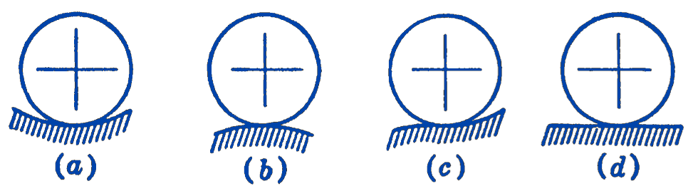
In (a) the cylinder rests on a concave surface; in (b) on a convex surface; in (c) on a point of inflection; and in (d) on a plane surface. Applying the principle of virtual displacements, it will be seen that all four of the positions are equilibrium positions, since the only active force is a vertical gravity force, and since the center of gravity of the cylinder moves horizontally for an infinitesimal rolling displacement of the cylinder. We can also relate these situations to the fact that the potential energy of the system must have a stationary value at the position of equilibrium. In (a), the potential energy of the system is seen to be a minimum, since the cylinder is in its lowest position, and work would have to be done on the cylinder to move it in either direction. In (b) the potential energy of the system is a maximum, since the cylinder is at the highest position, and work would be done by the system as it moved in either direction. The point of inflection of (c) corresponds to a stationary value, since the potential energy of the cylinder is neither a maximum nor a minimum.
It will also be recognized that the positions shown in Fig. 3-11 are physically somewhat different. In (a), we may say that we have stable equilibrium, since any movement away from the position of equilibrium sets up forces which will return the system to the equilibrium position, (b) and (c) are examples of unstable equilibrium, since any movement away from the position of equilibrium sets up forces which will move the system still further from the equilibrium position, and (d) illustrates neutral or indifferent equilibrium, in which motion of the system from the position of equilibrium does not affect the equilibrium of the system.
We can thus conclude that the maximum potential energy condition corresponds with the unstable condition, while the minimum potential energy condition corresponds with the stable condition.
The above considerations can be used to test an equilibrium position as to whether it is stable or unstable. It is only necessary to note whether the potential energy of the system increases or decreases as the system is moved from the position of equilibrium.
The conditions for equilibrium and the tests for stable and unstable equilibrium can be expressed analytically as follows. Suppose that for simplicity we consider a system whose displacement from a position of equilibrium can be described by one coordinate, \(x\). Let \(P\) be this position of equilibrium, and \(V_{P}\) the potential energy of the system at the position \(P\). Now, as \(x\) changes and we move away from the position of equilibrium, the potential energy of a conservative system will be some function of \(x\): \[ V=f(x). \]
If we now write the Maclaurin series expansion of this function about the point \(P\), we have :
\[ \begin{aligned} V & =V_{P}+x\left(\frac{d V}{d x}\right)_{P}+\frac{1}{2} x^{2}\left(\frac{d^{2} V}{d x^{2}}\right)_{P}+\cdots \\ V-V_{P} & =x\left(\frac{d V}{d x}\right)_{P}+\frac{1}{2} x^{2}\left(\frac{d^{2} V}{d x^{2}}\right)_{P}+\cdots \end{aligned} \]
By the theorem of virtual displacements, we know that the work done by the forces upon an arbitrary infinitesimal displacement from the point \(P\) is zero, if the point \(P\) is a position of equilibrium. Thus, if we choose an infinitesimal displacement \(d x\), then the corresponding \(d V\) would be zero for equilibrium. The analytical condition for equilibrium of the system at the point \(P\) thus becomes: \[ \left(\frac{d V}{d x}\right)_{P}=0. \]
The change in the potential energy of the system, in the region near the equilibrium position, is then given by:
\[ V-V_{P}=\frac{1}{2} x^{2}\left(\frac{d^{2} V}{d x^{2}}\right)+\cdots \]
since the term \(\left(\frac{d V}{d x}\right)_{P}\) is zero.
Thus by examining the sign of the second derivative, we determine whether the potential energy is increasing or decreasing as we move away from the equilibrium position, and hence whether the system is stable or unstable.
From the above considerations, we see that while the positions of equilibrium can be determined by the principle of virtual displacements by considering only the first-order terms of the small displacements, it is necessary to investigate the second-order terms in order to decide as to the stability or instability of the equilibrium position.
| Sign of \(\left(\frac{d^{2} \nu}{d x^{2}}\right)_{x=0}\) | Potential Energy \(V\) | Equilibrium Condition |
|---|---|---|
| \(+\) | minimum | stable |
| \(-\) | maximum | unstable |
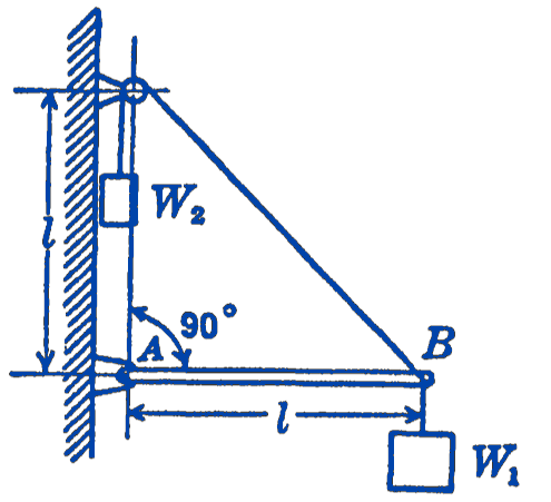
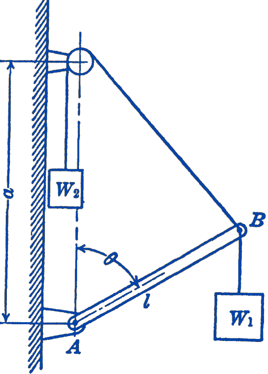
Example 1. A weight \(W_{1}\) is supported by a rigid, weightless bar, \(A B\), and a cable loaded by a weight \(W_{2}\), as shown in Fig. 3-12. Find the relationship between \(W_{1}\) and \(W_{2}\) for equilibrium of the system with the bar \(A B\) in a horizontal position, and determine whether this position of equilibrium is stable or unstable.
Solution. We shall work this problem in two ways, first by the principle of virtual displacements, and second by means of potential energy considerations.
First Method
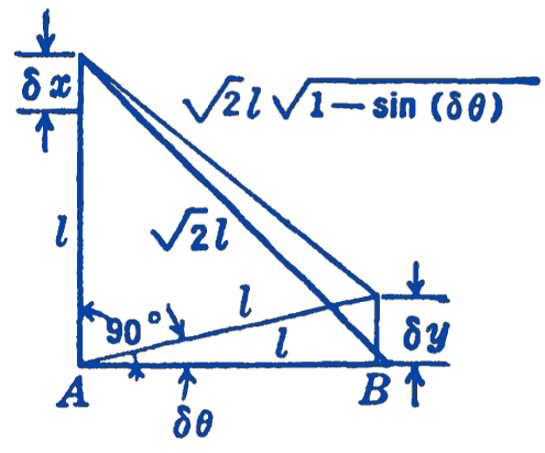
We take as a virtual displacement of the system a small lowering of the weight \(W_{2}\), which we shall call \(\delta x\). We can then find from the geometry of the system the distance through which \(W_{1}\) rises, \(\delta y\). \[ \begin{aligned} \delta x+\sqrt{2} l \sqrt{1-\sin (\delta \theta)} & =\sqrt{2} l \\ \sqrt{1-\sin (\delta \theta)} & =\frac{\sqrt{2} l-\delta x}{\sqrt{2} l} \\ \sin (\delta \theta) & =\frac{2 \sqrt{2} l(\delta x)-(\delta x)^{2}}{2 l^{2}} \end{aligned} \] also \[ \sin (\delta \theta)=\frac{(\delta y)}{l} ; \quad \delta y=l \sin (\delta \theta) \] so \[ \delta y=\sqrt{2}(\delta x)-\frac{(\delta x)^{2}}{2 l}. \] To find the equilibrium conditions, we note that the virtual work is zero, and that we can drop the second-order terms \((\delta x)^{2}\) in calculating this virtual work. \[ \begin{gathered} \delta W=W_{2}(\delta x)-W_{1}(\delta y)=0 \\ W_{2}(\delta x)-W_{1}[\sqrt{2}(\delta x)]=0 \\ W_{2}=\sqrt{2} W_{1} \end{gathered} \]
This answer can be very simply checked by equating the moments about the point \(A\) to zero, for equilibrium.
In order to investigate the stability of this equilibrium position, we must see whether it requires work to be done upon the system to move it from the position of equilibrium, or whether the system itself can do work as it moves from the position of equilibrium.
The work done by the system during the displacement \(\delta x\) from the position of equilibrium is: \[ \begin{aligned} & W_{2}(\delta x)-W_{1}(\delta y) \\ = & W_{2}(\delta x)-W_{1}\left[\sqrt{2}(\delta x)-\frac{(\delta x)^{2}}{2 l}\right] \end{aligned} \] Putting in the equilibrium condition \(W_{2}=\sqrt{2} W_{1}\) we have: \[ \begin{aligned} & \sqrt{2} W_{1}(\delta x)-\sqrt{2} W_{1}(\delta x)+W_{1} \frac{(\delta x)^{2}}{2} \\ = & +W_{1} \frac{(\delta x)^{2}}{2 l} \end{aligned} \]
Note that we have left only a second-order term \((\delta x)^{2}\) so that second-order terms must be retained to investigate such stability problems.
Since this work term is positive, we see that the system itself does work as it moves from the position of equilibrium, i.e., the potential energy would be decreasing, hence the position of equilibrium is unstable.
Second Method
We write down the expression for the potential energy of the system in a region close to the equilibrium position: \[ V=V_{P}-W_{2} x+W_{1}\left(\sqrt{2} x-\frac{x^{2}}{2 l}\right) \] where \(x\) is the downward displacement of \(W_{2}\) from the equilibrium position, and \(V_{P}\) is the potential energy of the system at the equilibrium position, measured from any arbitrary level.
The equilibrium condition is: \[ \begin{aligned} \left(\frac{d V}{d x}\right)_{x-0} & =0=-W_{2}+W_{1} \sqrt{2}-\frac{W_{1} x}{l} \\ W_{2} & =\sqrt{2} W_{1} \end{aligned} \]
The test for stability is:
\[ \left(\frac{d^{2} V}{d x^{2}}\right)_{x=0}=-\frac{W_{1}}{l}, \text { negative, hence unstable } \]
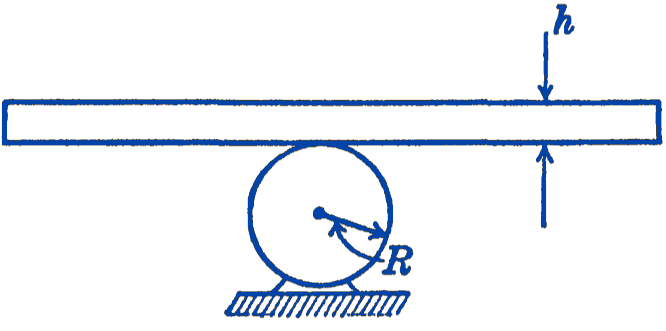
Example 2. A uniform plank of thickness \(h\) is balanced on top of a circular cylinder of radius \(R\) (Fig. 3). What is the relationship between \(h\) and \(R\) for stability of the equilibrium position, assuming that the plank rolls on the cylinder without sliding?
Solution. Consider a virtual displacement \(\delta \theta\) of the system consisting of the plank rolling on the cylinder (Fig. 4).
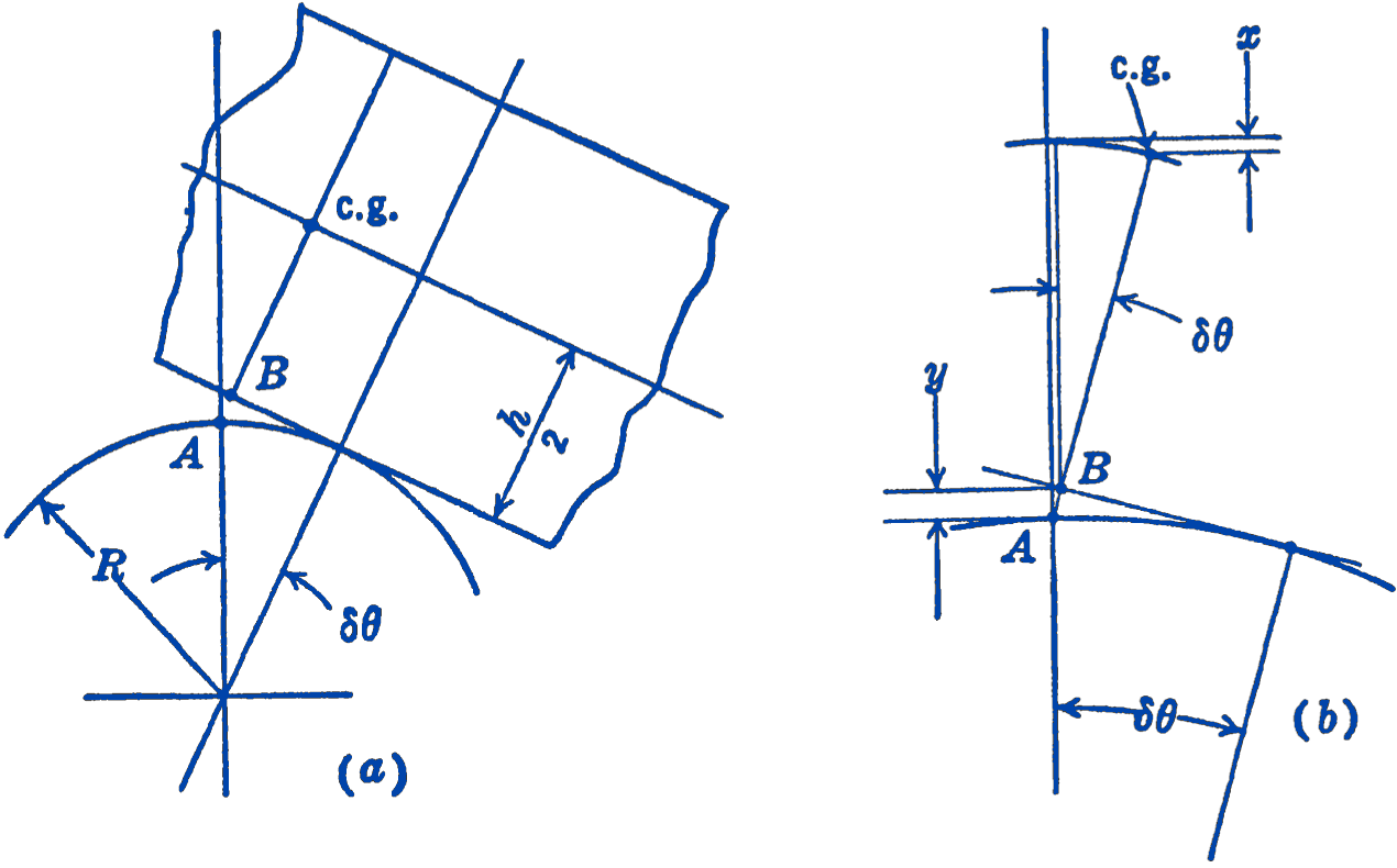
Originally, the points \(A\) and \(B\) coincide; after the virtual displacement the points \(A\) and \(B\) assume the positions shown in the diagrams. We wish to compute the total vertical movement of the center of gravity of the plank during the displacement \(\delta \theta\). If this vertical movement is upward, the equilibrium position is stable. If this vertical movement is downward, the equilibrium is unstable. To solve for the limiting condition, we find the relationship between \(h\) and \(R\) for which there will be no vertical movement of the c.g. In diagram (b) it will be seen that the total vertical motion can be considered as composed of two parts, one a downward component, due to the rotation of the plank, marked \(x\) in the diagram; and the other an upward component due to rolling of the plank, marked \(y\) in the diagram. The limiting condition for stable equilibrium will be determined by equating these two components.
From the figure, we have directly: \[ x=\frac{h}{2}[1-\cos (\delta \theta)]=\frac{h}{2}\left[1-1+\frac{1}{2}(\delta \theta)^{2}-\frac{1}{24}(\delta \theta)^{4}+\cdots\right]. \] By retaining second-order terms, but neglecting higher orders, we have: \[ x=\frac{h}{4}(\delta \theta)^{2}. \]
To find \(y\), note that in Fig. 5 the length \(y\) is less than \(A C\), but greater than the vertical component of \(A D\). We can show, however, that the difference between \(A C\) and \(A D \cos (\delta \theta\) ) involves only terms higher than second order, so that if we retain terms only through the second order we can say that \(y=A C\).
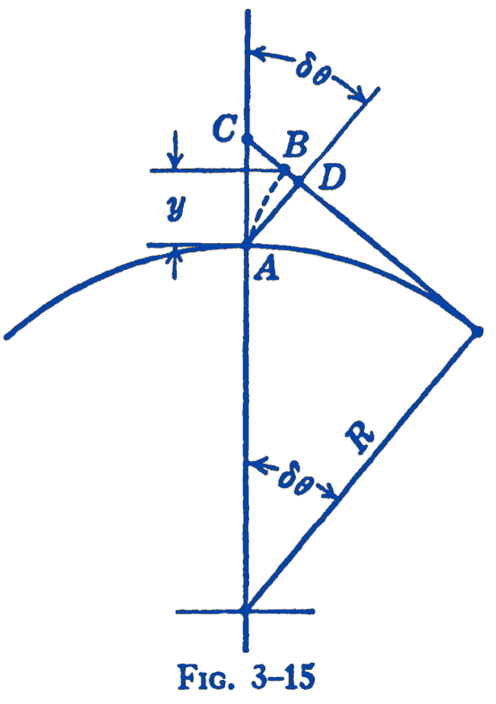
\[ \begin{aligned} \frac{R}{R+(A C)} & =\cos (\delta \theta) \\ (A C) & =R[\sec (\delta \theta)-1]=R\left[1+\frac{1}{2}(\delta \theta)^{2}+\frac{5}{24}(\delta \theta)^{4}+\cdots-1\right] \\ & =R\left[\frac{1}{2}(\delta \theta)^{2}+\text { higher order terms }\right] \\ A D \cos (\delta \theta) & =R[1-\cos (\delta \theta)] \cos (\delta \theta) \\ & =R\left[1-1+\frac{1}{2}(\delta \theta)^{2}-\frac{1}{24}(\delta \theta)^{4}+\cdots\right] \\ & =R\left[\frac{1}{2}(\delta \theta)^{2}+\text { higher order terms }\right]. \end{aligned} \] Therefore, to the second-order approximation: \[ y=A C=\frac{R}{2}(\delta \theta)^{2} \] For the limiting case of stable equilibrium, \[ \begin{aligned} x & =y \\ \frac{h}{4}(\delta \theta)^{2} & =\frac{R}{2}(\delta \theta)^{2} \\ R & =\frac{h}{2} \end{aligned} \]
For example, a \(2\ \mathrm{in}\) thick plank would require a cylinder of \(1\ \mathrm{in}\) radius. Any smaller cylinder would represent a case of unstable equilibrium.
3.6.1 PROBLEMS
1. A door can swing through \(360^{\circ}\) around an axis which makes an angle \(\alpha\) with the vertical, as shown in the figure. Show that the system has two positions of equilibrium, one of them stable, and the other unstable.
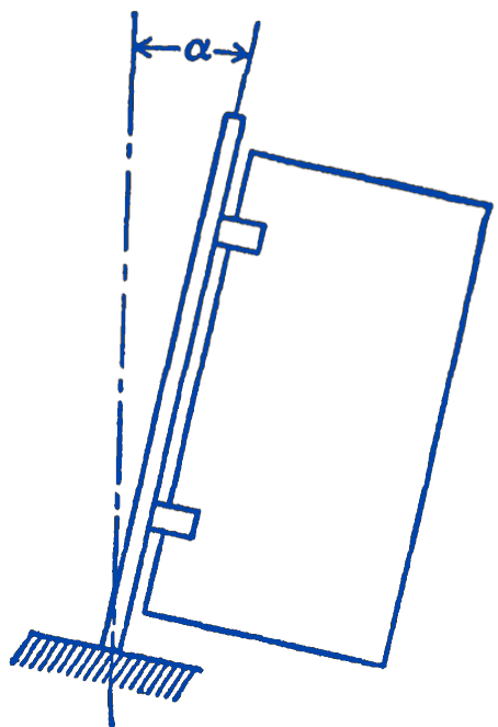
2. Referring to the previous problem, determine whether the equilibrium position of the uniform bar is stable or unstable.
Answer
Unstable
3. A homogeneous body is composed of a semi-cylinder and a rectangular parallelepiped, as shown in the figure. Find the maximum value of \(h\) consistent with stability of the system on the horizontal plane. The cylinder is assumed to roll on the plane without sliding.
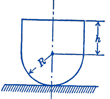
Answer
\(h=\sqrt{\frac{2}{3}} R\)
4. A rigid weightless bar \(A B\) supports a weight \(W_{1}\) and is supported by a cable which is loaded by a weight \(W_{2}\) as shown in the figure. The distance \(a\) is greater than the distance \(l\). Find all possible equilibrium positions of the system and investigate their stability.
Answer
\(\theta_{1}=\cos ^{-1}\left\{\frac{a^{2}\left[1-\left(\frac{W_{2}}{W_{1}}\right)^{2}\right]+l^{2}}{2 a l}\right\}\), \(\theta_{2}=0^{\circ}, \theta_{3}=180^{\circ}\)