A general relationship between the load, the shearing force, and the bending moment may be derived in the following way. Consider a beam with any load which is given by the function \(q(x)\), where \(q\) is a distributed load in pounds per foot which may vary in any way. In Fig. 1 is shown a free-body diagram of a portion of this beam of length \(d x\).

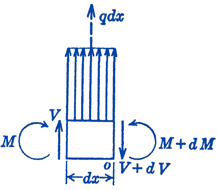
For equilibrium, we have: \[ \begin{aligned} & \sum F_{y}=0=V+q\, d x-(V+d V) \\ & \sum M_{o}=0=M+d M-M-V\, d x-(q\, d x)\left(\frac{d x}{2}\right) \end{aligned} \] From the first equation: \[ \bbox [5px,border:1px #f2f2f2;background-color:#f2f2f2]{q=\frac{d V}{d x}} \] And from the second equation, neglecting the second-order differential \((d x)(d x)\) : \[ \bbox [5px,border:1px #f2f2f2;background-color:#f2f2f2]{V=\frac{d M}{d x}} \]

These expressions give the relationship between the load, shearing force, and bending moment in a beam. The first expression states that the ordinate of the load diagram is equal to the slope of the shearing force diagram, while the second expression states that the ordinate of the shear force diagram is equal to the slope of the bending moment diagram. By the use of the second statement, the bending moment diagram can be constructed once the shearing force diagram is known. The value of the bending moment can be expressed in terms of the shearing force by integrating the second expression above to give: \[ \bbox [5px,border:1px #f2f2f2;background-color:#f2f2f2]{M=\int V\, d x+c} \] This states that the difference between the magnitude of the bending moment at two points of a beam is equal to the area of the shearing force diagram between those two points.

In the design of beams, one is usually most interested in finding the magnitude of the maximum bending moment. This maximum bending moment will occur at the point where the slope of the bending moment diagram is zero, and hence at the point where the shearing force diagram is zero. Each point in a beam where the shearing force diagram passes through zero should thus be examined as a possible point of maximum bending moment for the whole beam.

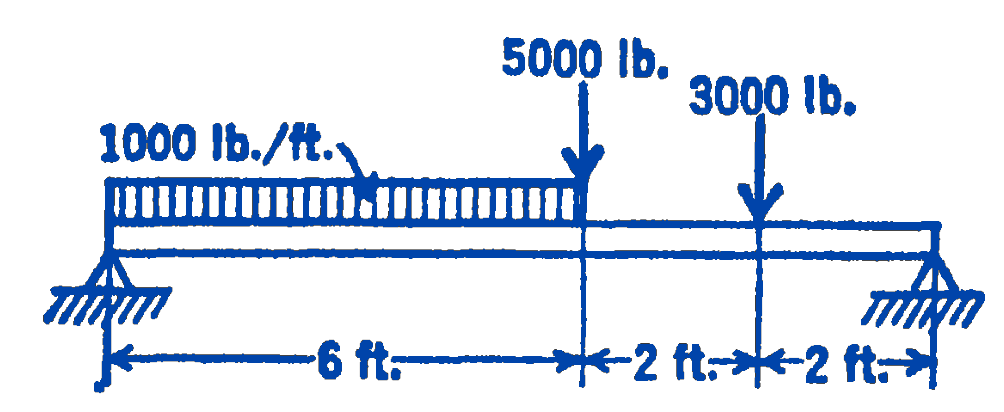
Example. Using the information derived above, find the maximum bending moment in the beam shown in Fig. 2.

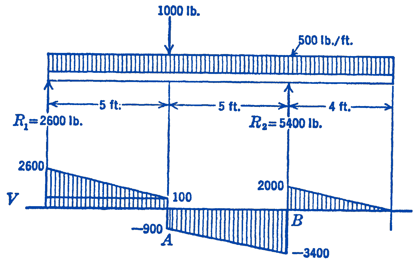
Solution. We first determine the reactions and plot the shearing force diagram by the previously described method. The relationship \(q=\dfrac{d V}{d x}\) tells us that where the load is uniformly distributed the slope of the shear force diagram is constant, and that where a concentrated load occurs there will be a discontinuity in the shear force diagram.

The shear force diagram crosses the zero axis at two points, \(A\) and \(B\), one of which must be the maximum bending moment for the entire beam. The magnitude of the bending moment at \(A\) is the area of the shear force diagram to the left of \(A\), and the magnitude of the bending moment at \(B\) is the area of the shear force diagram to the right of \(B\). These areas are:

\[ \begin{aligned} & \text { at } A:(2500)(5)\left(\frac{1}{2}\right)+(5)(100)=6750 \ \mathrm{ft}\cdot\mathrm{lb} \\ & \text { at } B: \quad-(2000)(4)\left(\frac{1}{2}\right)=-4000\ \mathrm{ft}\cdot\mathrm{lb} \end{aligned} \] Hence the maximum bending moment is the positive bending at \(A\) of \(6750\ \mathrm{ft}\cdot\mathrm{lb}\).

6.12.1 PROBLEMS

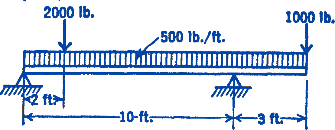
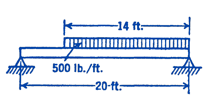
1. Find the bending moment diagram for the following beam, graphically, using a funicular polygon, and check the maximum value of bending moment in the beam.

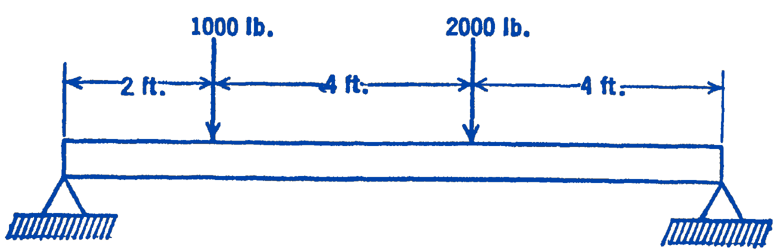
2. Using the method of the example in this section, construct the bending moment diagram and find the maximum bending moment for the beam shown below.

3. Same as the previous problem for the beam shown below.

4. Same as the previous problem for the beam shown below.