In some cases the load acting on a flexible cable is uniformly distributed along the length of the cable rather than along the horizontal. This is always the situation when the major load on the cable is its own weight, as for an electrical transmission line. In this problem the same differential equation derived above is valid: \[ \frac{d y}{d x}=\frac{W}{F_{h}} \] where now \[ W=w_{1} s \] where \(w_{1}\) is the weight per unit length of the cable, and \(s\) is the length of the cable from the lowest point to the point \(x, y\).

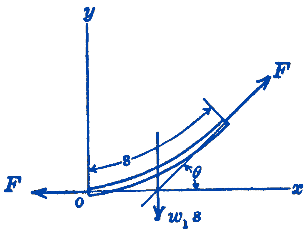
Expressing \(s\) in terms of \(x\) and \(y\) we have: \[ \frac{d s}{d x}=\sqrt{1+\left(\frac{d y}{d x}\right)^{2}}. \]

Since \[ \frac{d y}{d x}=\frac{w_{1} s}{F_{h}} \] this becomes \[ \begin{aligned} \frac{d s}{d x} & =\sqrt{1+\left(\frac{w_{1} s}{F_{h}}\right)^{2}} \\ x & =\int \frac{d s}{\sqrt{1+\left(\dfrac{w_{1} s}{F_{h}}\right)^{2}}} \end{aligned} \] From the integral tables we find: \[ x=\frac{F_{h}}{w_{1}} \sinh ^{-1} \frac{w_{1} s}{F_{h}}+C_{1} \]

when \(x=0, s=0\), therefore \(C_{1}=0\). Thus \[ \frac{w_{1} s}{F_{h}}=\sinh \frac{w_{1} x}{F_{h}} ; \quad s=\frac{F_{h}}{w_{1}} \sinh \frac{w_{1} x}{F_{h}} \]

Substituting this into the original differential equation, we get: \[ \begin{aligned} \frac{d y}{d x} & =\sinh \frac{w_{1} x}{F_{h}} \\ y & =\int \sinh \frac{w_{1} x}{F_{h}} d x=\frac{F_{h}}{w_{1}} \cosh \frac{w_{1} x}{F_{h}}+C_{2} \end{aligned} \] when \(x=0, y=0\) \[ 0=\frac{F_{h}}{w_{1}} \cosh 0+C_{2} ; \quad C_{2}=-\frac{F_{h}}{w_{1}} \ \] hence \[ \bbox [5px,border:1px #f2f2f2;background-color:#f2f2f2]{y=\frac{F_{h}}{w_{1}}\left(\cosh \frac{w_{1} x}{F_{h}}-1\right).} \] This equation gives the curve which will be assumed by the flexible cable hanging under its own weight. Such a curve is called a catenary.

The force in the cable can be found in the same way as for the parabolic cable, Equation (2) of the previous section becoming: \[ F=\sqrt{F_{h}^{2}+w_{1}^{2} s^{2}}=F_{h} \sqrt{1+\sinh ^{2} \frac{w_{1} x}{F_{h}}} \] since \[ \cosh ^{2} \alpha-\sinh ^{2} \alpha=1 \] this gives: \[ F=F_{h} \cosh \frac{w_{1} x}{F_{h}} \] for the case of a cable suspended from two supports at the same level. The maximum force will occur at the support, where \(x=\dfrac{l}{2}\), so \[ F_{\max }=F_{h} \cosh \frac{w_{1} l}{2 F_{h}} \] To find \(F_{h}\) we note that when \(x=\frac{l}{2}, y=f\). Introducing these values into the equation relating \(x\) and \(y\) gives: \[ f=\frac{F_{h}}{w_{1}}\left(\cosh \frac{w_{1} l}{2 F_{h}}-1\right) \]

This equation can in most practical problems be solved easily by trial and error.

6.15.1 PROBLEMS