Consider an area and an \(x y\) coordinate system in the plane of the area as shown in Fig. 1.

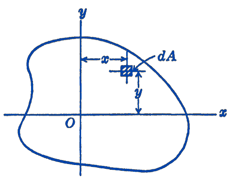
The integral \[\bbox [5px,border:1px #f2f2f2;background-color:#f2f2f2]{I_{x y}=\displaystyle \int_{A} x y\, d A}\] is called the product of inertia of the area with respect to the \(x y\) coordinate system. Integrals of this form often appear in the analysis of problems in dynamics and strength of materials and it will be necessary to evaluate such terms.

For some simple figures it will be possible to compute the product of inertia directly by integration. For more complex figures, the figure may be broken down into simpler elements for which the products of inertia are known or may be easily determined, and the total product of inertia will then be the sum of the products of inertia of the parts. For this purpose it will be desirable to have a parallel-axis theorem for the transfer of the product of inertia from one coordinate system to another.

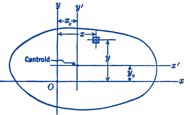
Suppose that the products of inertia \(I_{x_{c} y_{c}}\) of an area are known for rectangular axes located at the centroid of the area, as shown in Fig. 2. To find the product of inertia \(I_{x y}\) about any other parallel coordinate system, we have: \[ \begin{aligned} I_{x y} & =\int_{A}\left(x_{c}+x^{\prime}\right)\left(y_{c}+y^{\prime}\right)\,dA \\ & =\int_{A} x_{c} y_{c} d A+\int_{A} x^{\prime} y_{c} d A+\int_{A} y^{\prime} x_{c} d A+\int_{A} x^{\prime} y^{\prime} d A \end{aligned} \] The first term becomes \(x_{c} y_{c} A\), the second and third terms drop out, since the \(x^{\prime} y^{\prime}\) axes pass through the centroid of the area, and the last term is \(I_{x_{c} y_{c}}\), so that: \[ \bbox [5px,border:1px #f2f2f2;background-color:#f2f2f2]{I_{x y}=I_{x_{c} y_{c}}+x_{c} y_{c} A} \] If axes are to be transferred from one non-centroidal axis to a parallel non-centroidal axis, it should be noted that it will first be necessary to determine the product of inertia about a centroidal system as an intermediate step. The above expression for the transfer to parallel axes applies only when the \(x^{\prime} y^{\prime}\) axes are at the centroid of the area.

Since the terms \(x\) and \(y\) appearing in the expression for the product of inertia may be either positive or negative, the product of inertia itself may be either positive or negative. That portion of the area which lies in the first quadrant will give a positive product of inertia, that portion which lies in the second quadrant will give a negative product of inertia, etc. The sign of the total product of inertia can usually be checked by inspection, since it will depend upon the relative portions of the area which lie in the various quadrants. If either the \(x\) or the \(y\) axis is an axis of symmetry for the figure, then \(I_{x y}=0\), since there will be a negative \(x y\, d A\) term to cancel each positive \(x y\, d A\) term. This fact can often be used, in combination with the parallel-axis theorem, to find the product of inertia without integration.

Example. Find the product of inertia of the area of a right triangle with respect to centroidal axes parallel to the base and altitude.

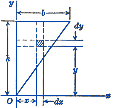
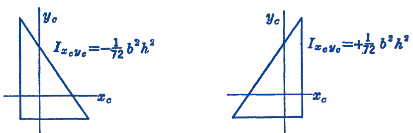
Solution. This problem may be solved most directly by first finding the product of inertia with respect to the \(x y\) system shown in Fig. 3 by integration, and then by using the transfer theorem to find the centroidal product of inertia. \[ \begin{aligned} I_{x y}&=\int_{0}^{h} \left(\int_{0}^{\frac{b}{h}y} x y\, d x\right) d y \\ & =\left.\int_{0}^{h} y\left(\frac{x^{2}}{2}\right)\right|_{0} ^{\frac{b}{h} y} d y=\int_0^h \frac{y}{2} \left(\frac{by}{h}\right)^2dy\\ &=\frac{b^{2}}{2 h^{2}} \int_{0}^{h} y^{3} d y=\left.\frac{b^{2}}{2 h^{2}} \frac{y^{4}}{4}\right|_{0} ^{h} \\ & =\frac{1}{8} b^{2} h^{2} \end{aligned} \] From the transfer theorem, we have: \[ \begin{aligned} I_{x_c y_c} & =I_{x y}-\left(x_{c}\right)\left(y_{c}\right) A\\ &=\frac{1}{8} b^{2} h^{2}-\left(\frac{2}{3} h\right)\left(\frac{1}{3} b\right)\left(\frac{1}{2} b h\right) \\ & =\frac{1}{8} b^{2} h^{2}-\frac{1}{9} b^{2} h^{2}\\ &=\frac{1}{72} b^{2} h^{2} \end{aligned} \] Note that the problem statement does not lead to a unique answer, since the sign of \(I_{x_c y_c}\) depends upon the orientation (Fig 4).