Most of the forces with which we have been dealing have been assumed to be concentrated at one point. Our only exception, so far, has been the case of uniformly distributed gravity forces. There are a number of other common situations in which the forces are distributed throughout a volume or over an area. We know, for example, that it is impossible in nature to achieve a load which is concentrated at just one point. The inevitable deformation of loaded surfaces in contact will insure that the load is in actuality distributed over some small area, rather than being concentrated at a point. This distribution of load over an area is in general a desirable thing, since for engineering materials there is an upper limit to the load per unit area which can be safely supported, before a rupture or fracture of the material would occur. If a given load is to be supported by a surface, it is sometimes necessary to take special care to see that the load is distributed over an appreciable area, to avoid excessive unit loadings.
An example of such a loading is the beam shown in Fig. 1.
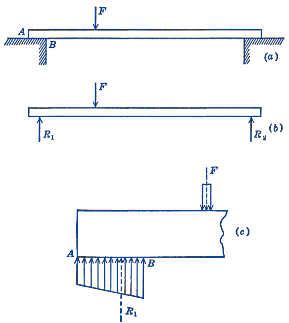
In Fig. 1a the fact that the beam is supported at the two ends and loaded by a concentrated load between the supports is indicated. In (b) the free-body diagram of the beam is shown, and the loads and reactions have been indicated, as in the preceding chapters, as concentrated loads. In (c) a more exact picture of the actual state of affairs is shown. Both the externally applied load \(F\) and the reactions \(R_{1}\) and \(R_{2}\) at the supports are in reality distributed systems of parallel forces. The force between the beam and the supporting surface is shown to be distributed over a length \(A B\) of the beam, instead of at a point. Because of the manner in which the beam has deformed, it is also likely that this force is non-uniformly distributed over the distance \(A B\), and that it is greater at \(B\) than at \(A\). We have accordingly shown, as a first approximation, a linear variation of force along the length \(A B\). This diagram, which indicates the way the force varies along the length of the beam is called the force diagram, and an ordinate of this diagram, a force per unit length, is called the force intensity. It will be seen that the area of the force diagram is equal to the resultant force of the parallel force system, and that this resultant passes through the centroid of the area of the force diagram. In this way we can reduce the distributed force system, for statical purposes, to a single force acting at a determinate point.
In the above example we have considered only those variations in the intensity of the force along the length of the beam. In some problems the variations of this force intensity across the width of the beam must also be considered. Such a three-dimensional force distribution is shown in Fig. 2.
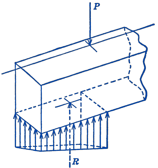
In this case the load \(P\) is located off of the centerline of the beam, so that the reaction force intensities are greater along the back portion of the beam than they are along the front edge of the beam.
The reaction forces thus form, as in Fig. 2, a system of parallel forces in space. Instead of a force intensity, we now speak of a force per unit area, called a pressure or a stress. This non-uniformly distributed force system in space could thus be replaced, for statical purposes, by a single resultant force whose magnitude is equal to the volume of the pressure diagram, and which passes through the centroid of that volume.
Example. One end of a beam is built into a wall as shown in Fig. 3a, while the other end is loaded by a concentrated force \(P\). Assuming that the variation of the force intensity of the reaction forces on the beam is as shown in (b), find the maximum force intensities \(p_{1}\) and \(p_{2}\).
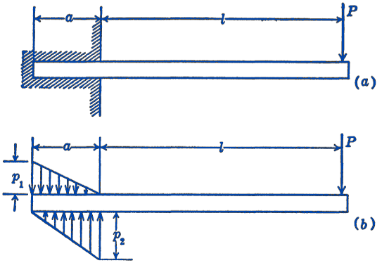
Solution. We can replace the distributed loads shown by resultant forces acting through the centroids of the force intensity diagrams, as shown in (c).
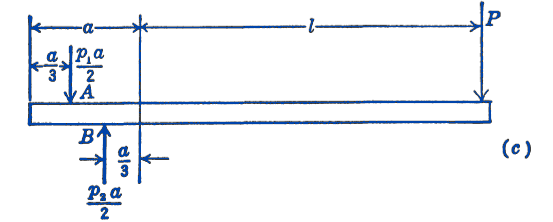
Taking moments about the point \(A\), we have for equilibrium: \[ \begin{aligned} \sum M_{A} & =0=\left(\frac{a}{3}\right)\left(\frac{p_{2} a}{2}\right)-\left(l+\frac{2}{3} a\right) P \\ p_{2} \frac{a^{2}}{6} & =\left(l+\frac{2}{3} a\right) P \\ p_{1} & =\frac{6 P}{a^{2}}\left(l+\frac{2}{3} a\right) \end{aligned} \] also \[ \begin{aligned} \sum M_{B} & =0=\left(\frac{a}{3}\right)\left(\frac{p_{1} a}{2}\right)-\left(l+\frac{1}{3} a\right) P \\ p_{1} \frac{a^{2}}{6} & =\left(l+\frac{1}{3} a\right) P \\ p_{1} & =\frac{6 P}{a^{2}}\left(l+\frac{1}{3} a\right) \end{aligned} \] As a check equation, we can write the force summation equation: \[ \begin{aligned} \sum F_{y}=0 & =-\frac{p_{1} a}{2}+\frac{p_{2} a}{2}-P \\ & =-\frac{3 P}{a}\left(l+\frac{1}{3} a\right)+\frac{3 P}{a}\left(l+\frac{2}{3} a\right)-P \\ & =-\frac{3 P l}{a}-P+\frac{3 P l}{a}+2 P-P=0 \end{aligned} \]
4.9.1 PROBLEMS
1. A beam supports a concentrated load of \(100 \mathrm{lb}\) and is supported as shown in the figure. Assuming that the reaction forces at the support are uniformly distributed over the width of the support, find the intensity of the force at the two supports.
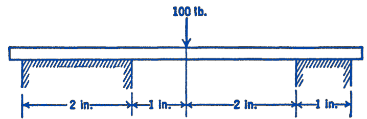
Answer
27.8 lb per in., 44.5 lb per in.
2. The load on a beam varies linearly from zero at one end to a load \(p\) per unit length of the beam at the other end. If the reaction \(R\) at the heavily loaded end of the beam is not to exceed \(1500\ \mathrm{lb}\), what is the maximum total load that can be carried by the beam?
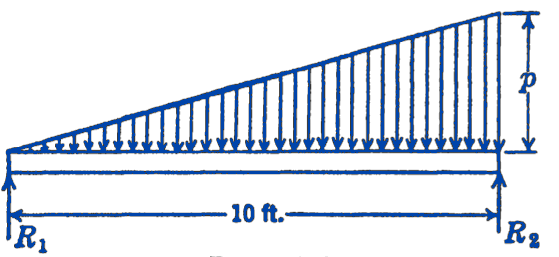
Answer
2250 lb
3. A beam is loaded and supported as shown in the diagram. Assuming that the reaction force diagram has a trapezoidal form, find the reaction force intensities.
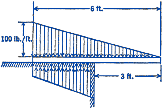
Answer
Max. intensity \(=200 \ \mathrm{lb}\) per ft