In a stressed body, the components of stress generally vary from point to point. These variations are not arbitrary; they are governed by Newton’s second law of motion. By applying this law to an infinitesimal element, we can find the governing equations for the variation of stress within a body.
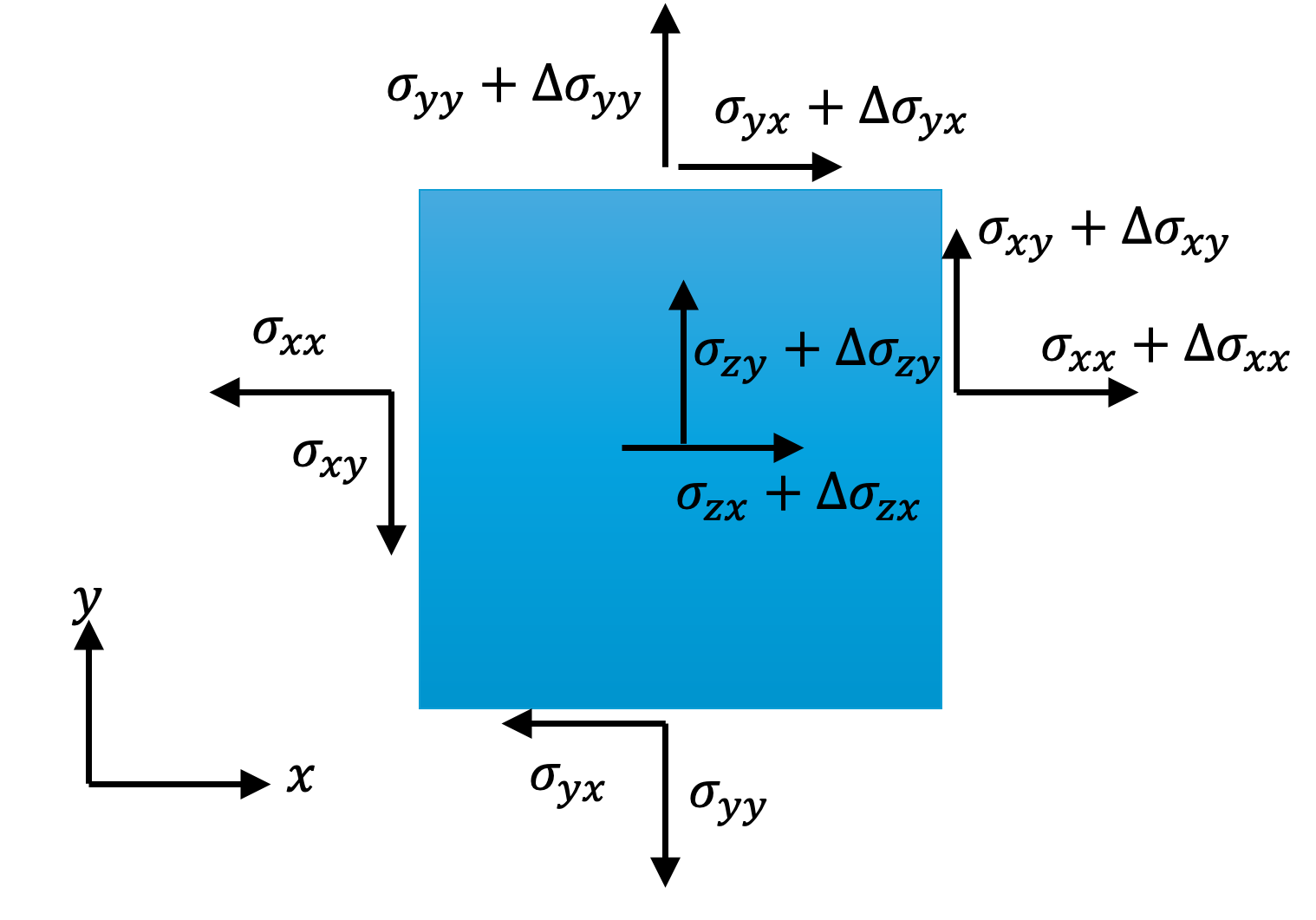
Consider an element with dimensions \(\Delta x\), \(\Delta y\), and \(\Delta z\). Stress components act on each face of this element. On each face of this cuboidal element, the stress components may differ from those on the opposite face. For example, if the xx-component of stress on one face is \(\sigma_{xx}\), then on the opposite face it will be taken as \(\sigma_{xx}+\Delta \sigma_{xx}\).
Let \(\mathbf{b}\) be the body force per unit mass. For example, if we consider only the gravity, then \(b=g\), where \(g\) is the gravitational acceleration. Therefore, the \(x\)-component of the force due to body force is \[ \rho b_x \Delta V=\rho b_x (\Delta x \Delta y\Delta z). \]where \(\rho\) is the mass-density at the point.
Now, summing the forces acting in the xxx-direction due to stresses on all faces and the body force, and applying Newton’s second law \(\sum F_x = m a_x\) gives \[ \begin{aligned} & \underbrace{(\sigma_{xx}+\Delta \sigma_{xx})\Delta y \Delta z}_{\text{on face at } x+\Delta x} - \underbrace{\sigma_{xx}\Delta y \Delta z}_{\text{on face at } x} \\ + & \underbrace{(\sigma_{yx}+\Delta \sigma_{yx})\Delta x \Delta z}_{\text{on face at } y+\Delta y} - \underbrace{\sigma_{yx}\Delta x \Delta z}_{\text{on face at } y} \\ + & \underbrace{(\sigma_{zx}+\Delta \sigma_{zx})\Delta x \Delta y}_{\text{on face at } z+\Delta z} - \underbrace{\sigma_{zx}\Delta x \Delta y}_{\text{on face at } z} \\ + & \underbrace{\rho b_x \Delta x \Delta y \Delta z}_{\text{body force}} = \underbrace{(\rho \Delta x \Delta y \Delta z)}_{m} a_x \end{aligned} \] After simplification and dividing both sides by the volume \(\Delta x \Delta y \Delta z\), we obtain: \[ \frac{\Delta \sigma_{xx}}{\Delta x}+\frac{\Delta \sigma_{yx}}{\Delta y}+\frac{\Delta \sigma_{zx}}{\Delta z}+\rho b_x=\rho a_x \] In the limit as \(\Delta x\to 0\), \(\Delta y\to 0\), and \(\Delta z\to 0\), the finite difference ratios become partial derivatives: \[ \frac{\partial \sigma_{xx}}{\partial x}+\frac{\partial \sigma_{yx}}{\partial y}+\frac{\partial \sigma_{zx}}{\partial z}+\rho b_x=\rho a_x \] By repeating this process for the y and z directions (\(\sum F_y =m a_y\) and \(\sum F_z=m a_z\)), we arrive at the full set of equations: \[ \begin{aligned} \frac{\partial \sigma_{xx}}{\partial x}+\frac{\partial \sigma_{yx}}{\partial y}+\frac{\partial \sigma_{zx}}{\partial z}+\rho b_x=\rho a_x \\ \frac{\partial \sigma_{xy}}{\partial x}+\frac{\partial \sigma_{yy}}{\partial y}+\frac{\partial \sigma_{zy}}{\partial z}+\rho b_y=\rho a_y \\ \frac{\partial \sigma_{xz}}{\partial x}+\frac{\partial \sigma_{yz}}{\partial y}+\frac{\partial \sigma_{zz}}{\partial z}+\rho b_z=\rho a_z \end{aligned} \] These three equations can be written concisely as: \[ \boxed{ \sum_{j=1}^3\frac{\partial \sigma_{ji}}{\partial x_j}+\rho b_i=\rho a_i \qquad (i=1, 2, 3)} \] This is also commonly written in vector or tensor notation as: \[ \nabla \cdot \boldsymbol{\sigma}+\rho \mathbf{b}=\rho\mathbf{a} \] which means \[ \begin{aligned} &{\left[\begin{array}{lll}\frac{\partial}{\partial x} & \frac{\partial}{\partial y} & \frac{\partial}{\partial z}\end{array}\right] \left[\begin{array}{lll}\sigma_{x x} & \sigma_{x y} & \sigma_{x y} \\ \sigma_{y x} & \sigma_{y y} & \sigma_{y y} \\ \sigma_{z x} & \sigma_{z y} & \sigma_{z z}\end{array}\right]+\rho\left[\begin{array}{lll}b_x & b_y & b_z\end{array}\right]} \\ & \qquad=\rho\left[\begin{array}{lll}a_x & a_y & a_y\end{array}\right]\end{aligned} \] This equation is known as Cauchy’s First Law of Motion.