Consider a two-dimensional, plane stress problem involving a long rectangular beam subjected to uniform tensile forces \(p\) at both ends, as shown below.
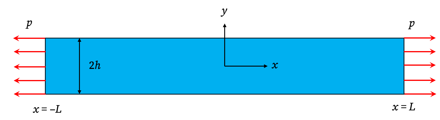
This case can be viewed as a Saint-Venant approximation of a more general situation with nonuniform end loading. In this interpretation, the actual distributed end tractions are replaced by statically equivalent uniform forces, and the resulting solution is valid in regions sufficiently far from the loaded ends.
Boundary Conditions
The boundary conditions for this problem may be written as
\[ \big(\sigma_x\big)_{x=\pm L} = p, \qquad \big(\sigma_y\big)_{y=\pm h} = 0, \qquad \big(\tau_{xy}\big)_{y=\pm h} = \big(\tau_{xy}\big)_{x=\pm L} = 0. \]
The Airy Stress Function
Because the boundary tractions are constant along each edge, we expect the stress field to be uniform. Therefore, we can assume a second-order Airy stress function of the form
\[ \phi = a_{02} y^2. \]
From this expression, the stress components become
\[ \sigma_x = 2a_{02}, \qquad \sigma_y = 0, \qquad \tau_{xy} = 0. \]
Applying the boundary condition \(\sigma_x = p\) at \(x = \pm l\) gives
\[ a_{02} = \frac{p}{2}. \] and \[ \phi =\frac{p}{2}y^2. \] Hence, the complete stress field is
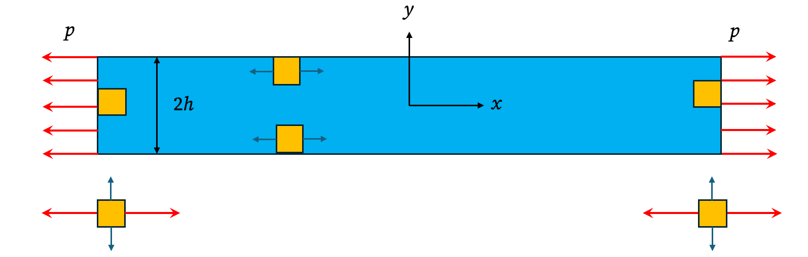
\[ \sigma_x = p, \qquad \sigma_y = \tau_{xy} = 0. \]
All boundary conditions are identically satisfied, and this uniform field represents a state of uniaxial tension.
Associated Displacement Field
Next, we determine the displacement field corresponding to this uniform stress state.
Using Hooke’s law for plane stress, the strains are given by \[ \varepsilon_x = \frac{1}{E}(\sigma_x - \nu\sigma_y) = \frac{p}{E}, \qquad \varepsilon_y = \frac{1}{E}(\sigma_y - \nu\sigma_x) = -\,\frac{\nu p}{E}. \] \[ \tau_{xy}=0 \]
From the strain–displacement relations, \[ \varepsilon_x = \frac{\partial u}{\partial x}, \qquad \varepsilon_y = \frac{\partial v}{\partial y}, \] we obtain the displacement gradients: \[ \frac{\partial u}{\partial x} = \frac{p}{E}, \qquad \frac{\partial v}{\partial y} = -\,\frac{\nu p}{E}. \]
Integrating these expressions with respect to their respective variables gives \[ u = \frac{p}{E}x + f(y), \qquad v = -\,\frac{\nu p}{E}y + g(x), \]
where \(f(y)\) and \(g(x)\) are “constants” of integration and will be determined from the shear strain relation.
Determination of f(y) and g(x)
For plane stress, the shear strain is related to the displacements by \[ \gamma_{xy} = \frac{\partial u}{\partial y} + \frac{\partial v}{\partial x}. \]
Since \(\tau_{xy} = 0\), Hooke’s law gives \(\gamma_{xy} = 0\), and therefore \[ \frac{\partial u}{\partial y} + \frac{\partial v}{\partial x} = 0. \]
Substituting the expressions for u and v yields \[ f'(y) + g'(x) = 0. \]
Because each side depends on a different variable, both must be constant: \[ g'(x) = c, \qquad f'(y) = -\,c. \]
Integrating, we find \[ f(y) = -\,c\,y + u_0, \qquad g(x) = c\,x + v_0, \]
where \(c\) represents a rigid-body rotation, and \(u_0, v_0\) are rigid translations in the \(x\)- and \(y\)-directions, respectively.
Final Form of the Displacement Field
Substituting these expressions into the earlier results gives the complete displacement field: \[ u = \frac{p}{E}x - c\,y + u_0, \qquad v = -\,\frac{\nu p}{E}y + c\,x + v_0. \]
The constants \(c, u_0,\) and \(v_0\) correspond to rigid-body motion and do not contribute to strain or stress. Therefore, the physical displacements are determined only up to an arbitrary rigid-body translation and rotation.
To determine \(c, u_0\) and \(v_0\), we need to apply an additional condition. For example, we can assume that the center of the beam does not move: \(u(0,0)=v(0,0)=0\).