We will now apply the Airy stress function method to one of the most fundamental problems in solid mechanics: determining the stress state within a prismatic beam subjected to a pure bending moment. While the solution is well-known from elementary mechanics of materials, deriving it through the theory of elasticity provides a more rigorous validation of the result and highlights the assumptions involved.

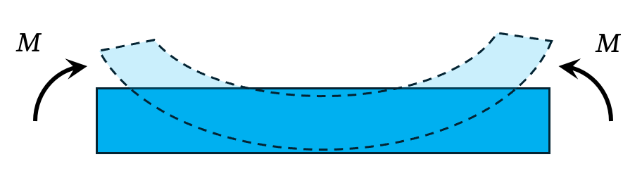
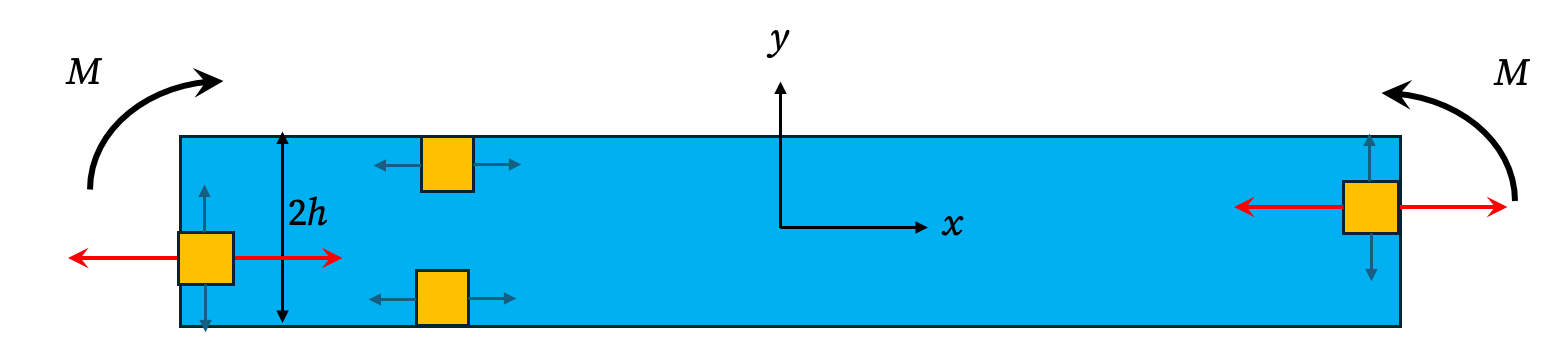
Consider a straight rectangular beam of length \(L\), height \(h\), and width \(b\). We establish a coordinate system with the x-axis along the centroidal axis of the beam, and the y-axis in the direction of its height. The beam occupies the region defined by \(-L/2 \le x \le L/2\) and \(-h/2 \le y \le h/2\). The beam is subjected to a pure bending moment, \(M\), at both ends.

Step 1: Assumptions and Boundary Conditions

Before seeking a solution, it is imperative to state our initial assumptions and then precisely define the conditions that our stress field must satisfy on all surfaces of the body.

1. The Plane Stress Assumption

A typical beam is a structure that is long relative to its cross-sectional dimensions, and its width (\(b\)) is often comparable to or not dramatically larger than its height (\(h\)). Furthermore, it is loaded only in the xy-plane. Because the beam is not very thick in the z-direction (the width) and there are no forces applied to the faces at \(z=\pm b/2\), it is physically reasonable to assume that the stress components acting in the z-direction are negligible throughout the body. Therefore, we assume: \[ \sigma_z = \tau_{xz} = \tau_{yz} = 0 \] This is precisely the definition of a plane stress state. This assumption allows us to use the two-dimensional elasticity framework we have developed.

2. Formulation of the Boundary Conditions

Now we can state the conditions on the boundaries of our 2D model.

• Conditions on the Top and Bottom Surfaces (\(y = \pm h/2\)): The top and bottom surfaces are free from any applied forces. This means there can be no normal stress (no vertical pressure) and no shear stress (no horizontal friction) acting on these surfaces. \[ \big(\sigma_y\big)_{y=h/2}= 0 \] \[ \big(\tau_{xy}\big)_{y=\pm h/2} = 0 \]
• Conditions on the Ends (\(x = \pm L/2\)): The resultant of the stress distribution at each end must be equivalent to a pure moment, \(M\). This implies three distinct integral conditions:
  • No Net Axial Force: \[ \int_{-h/2}^{h/2} \big(\sigma_x\big)_{x=\pm L/2}\ b \, dy = 0 \]
  • No Net Shear Force: \[ \int_{-h/2}^{h/2} \big(\tau_{xy}\big)_{x=\pm L/2}\ \overbrace{b \, dy}^{dA} = 0 \]
  • Net Bending Moment: Adopting the convention that a positive \(M\) causes tension for \(y>0\): \[ \int_{-h/2}^{h/2} \big(\sigma_x\big)_{x=\pm L/2} \cdot y \ \overbrace{b \, dy}^{dA} = -M \]

Step 2: Proposing a Form for the Airy Stress Function

With our conditions specified, we now seek an Airy stress function \(\phi\) that satisfies the biharmonic equation, \(\nabla^4\phi = 0\).

Let’s assume \(\sigma_y=0\) everywhere, not just on the boundaries. But why? Here is the line of reasoning:

1. We know from the boundary conditions that \(\sigma_y=0\) on the top and bottom surfaces (\(y=\pm h/2\)).
2. There are no body forces (like gravity) acting in the y-direction within the beam.
3. There is no mechanism in this pure bending problem that would suggest a vertical stress should develop internally.
4. Therefore, we can propose that the simplest possible solution that satisfies the boundary conditions is one where \(\sigma_y\) and \(\tau_{xy}\) are zero everywhere inside the beam, not just on the surfaces.

Let us test this hypothesis. If this simple stress state can be made to satisfy all the remaining boundary conditions, then by the principle of uniqueness of solution in elasticity, it must be the correct solution.

Translating this hypothesis into conditions on \(\phi\):

• If \(\sigma_y = \dfrac{\partial^2\phi}{\partial x^2} = 0\) everywhere, then \(\phi\) can at most be a linear function of \(x\). It can be written as \(\phi(x,y) = x f(y) + g(y)\).
• If \(\tau_{xy} = -\dfrac{\partial^2\phi}{\partial x \partial y} = 0\) everywhere, then the derivative of our form for \(\phi\) must be zero: \(-\frac{\partial}{\partial y}(f(y)) = 0\). This implies that \(f(y)\) must be a constant.
• Combining these, our function must have the form \(\phi(x,y) = (\text{constant}) \cdot x + g(y)\). However, the bending problem is symmetric about \(x=0\), so we expect the stresses to be independent of \(x\). A constant stress from the \(x\) term would violate the moment condition. The simplest possible form that respects the physics is to assume \(\phi\) is a function of \(y\) only.

We therefore propose a polynomial in \(y\) as our candidate solution: \[ \phi(y) = Ay^3 + By^2 + Cy + D \] This is a third-degree polynomial, so it automatically satisfies the biharmonic equation \(\nabla^4\phi=0\).

Step 3: Applying the Boundary Conditions to the Proposed Solution

Let’s find the stresses from our proposed \(\phi\) and see if they can satisfy all the conditions. \[ \sigma_x = \frac{\partial^2 \phi}{\partial y^2} = 6Ay + 2B \] \[ \sigma_y = \frac{\partial^2 \phi}{\partial x^2} = 0 \] \[ \tau_{xy} = -\frac{\partial^2 \phi}{\partial x \partial y} = 0 \] Our hypothesis immediately satisfies the conditions for \(\sigma_y\) and \(\tau_{xy}\) on the top and bottom surfaces, and also satisfies the condition of zero net shear force at the ends. We now check the remaining two end conditions to find the constants A and B.

Applying the No Axial Force Condition: \[ \int_{-h/2}^{h/2} \sigma_x (b \, dy) = \int_{-h/2}^{h/2} (6Ay + 2B) b \, dy = b \left[ 3Ay^2 + 2By \right]_{-h/2}^{h/2} = 2Bbh = 0 \] Since \(b\) and \(h\) are non-zero, this requires that B = 0.

Applying the Net Bending Moment Condition: With B=0, our normal stress is now just \(\sigma_x = 6Ay\). \[ \int_{-h/2}^{h/2} (\sigma_x \cdot y) (b \, dy) = \int_{-h/2}^{h/2} (6Ay \cdot y) b \, dy = 6Ab \int_{-h/2}^{h/2} y^2 dy = -M \] \[ 6Ab \left[ \frac{y^3}{3} \right]_{-h/2}^{h/2} = 2Ab \left( (h/2)^3 - (-h/2)^3 \right) = \frac{Abh^3}{2} = - M \] We can now solve for the constant A: \[ A =- \frac{2M}{bh^3} \] Recalling that the moment of inertia for a rectangular cross-section is \(I = \dfrac{bh^3}{12}\), we can write A in terms of I: \[ A = -\frac{2M}{12I} = -\frac{M}{6I} \]

Step 4: The Final Solution and Verification

We have successfully found all the coefficients based on our initial hypothesis. The Airy stress function for pure bending is: \[ \phi(y) = -\frac{M}{6I} y^3 \] From this function, we derive the final stress components: \[ \sigma_x = -\frac{M}{I} y \] \[ \sigma_y = 0 \] \[ \tau_{xy} = 0 \] This solution, derived from our educated guess that \(\sigma_y\) and \(\tau_{xy}\) were zero everywhere, successfully satisfies all the boundary conditions of the problem. This justifies our initial hypothesis and provides the classic flexure formula, rigorously derived from the theory of elasticity.

Step 3: Deriving the Displacement Field (\(u\), \(v\))

To find the displacements, we must integrate the strain-displacement relations, using the strains determined from our stress field via Hooke’s Law for plane stress.

1. Find the Strains: \[ \epsilon_{xx} = \frac{\sigma_{xx}}{E} = -\frac{My}{EI} \] \[ \epsilon_{yy} = -\frac{\nu \sigma_{xx}}{E} = \frac{\nu My}{EI} \] \[ \gamma_{xy} = \frac{\sigma_{xy}}{G} = 0 \]

2. Integrate the Strain-Displacement Relations: We start with \(\epsilon_{xx} = \dfrac{\partial u}{\partial x}\). Integrating with respect to \(x\) gives: \[ u(x,y) = \int -\frac{My}{EI} dx = -\frac{Mxy}{EI} + f(y) \] where \(f(y)\) is an arbitrary function of \(y\) that acts as an integration “constant”.

Next, from \(\epsilon_{yy} = \dfrac{\partial v}{\partial y}\): \[ v(x,y) = \int \frac{\nu My}{EI} dy = \frac{\nu My^2}{2EI} + g(x) \] where \(g(x)\) is an arbitrary function of \(x\).

3. Use the Shear Strain to Couple the Equations: We use the final relation, \(\gamma_{xy} = \frac{\partial u}{\partial y} + \frac{\partial v}{\partial x} = 0\), to find the unknown functions \(f(y)\) and \(g(x)\). \[ \frac{\partial}{\partial y}\left(-\frac{Mxy}{EI} + f(y)\right) + \frac{\partial}{\partial x}\left(\frac{\nu My^2}{2EI} + g(x)\right) = 0 \] \[ \frac{Mx}{EI} + f'(y) + g'(x) = 0 \] Rearranging this equation to separate variables: \[ g'(x) + \frac{Mx}{EI} = -f'(y) \] The left side is a function of \(x\) only, while the right side is a function of \(y\) only. The only way this equality can hold for all \(x\) and \(y\) is if both sides are equal to the same constant, say \(C_1\).

• \(g'(x) = - \dfrac{Mx}{EI}+C_1 \implies g(x) = - \dfrac{Mx^2}{2EI} + C_1x+ C_2\)
• \(f'(y) = -C_1 \implies f(y) = -C_1y + C_3\)

4. Assemble and Constrain Rigid Body Motion: Substituting these back, the general displacement field is: \[ u(x,y) = \frac{Mxy}{EI} - C_1y + C_3 \] \[ v(x,y) = -\frac{\nu My^2}{2EI} - \frac{Mx^2}{2EI} + C_1x + C_2 \] The constants \(C_1, C_2, C_3\) represent rigid body motion. To find them, we must fix the beam in space. Let’s enforce that the origin (\(x=0, y=0\)) does not translate, and that the slope of the neutral axis is zero at the origin. * \(u(0,0) = 0 \implies C_3 = 0\) * \(v(0,0) = 0 \implies C_2 = 0\) * \(\dfrac{\partial v}{\partial x}\bigg|_{x=0, y=0} = \left[ -\dfrac{Mx}{EI} + C_1 \right]_{x=0} = C_1 = 0\)

All three constants are zero. The final displacement field is: \[ u(x,y) = \frac{Mxy}{EI} \] \[ v(x,y) = -\frac{Mx^2}{2EI} - \frac{\nu My^2}{2EI} \]