Now let’s analyze the stress and displacement fields in a prismatic cantilever beam subjected to a concentrated transverse force. This case is fundamentally different from pure bending because the presence of a transverse force necessitates the existence of an internal shear force that varies along the beam’s length. It is this shear that will prove to be the source of the non-planar deformation.
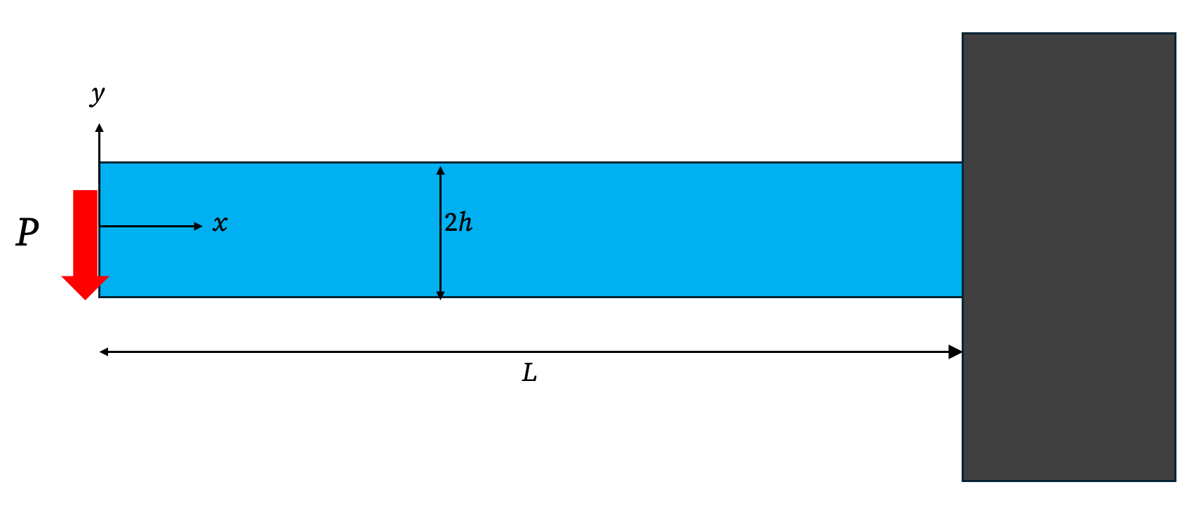
Consider a straight rectangular beam of length \(L\), height \(h\), and width \(b\). The beam is fixed at the end \(x=0\) and is free at the end \(x=L\). A concentrated vertical force, \(P\), acts downwards at the free end.
Step 1: Assumptions and Boundary Conditions
1. The Plane Stress Assumption
As with the pure bending case, the beam is slender, and the loading is confined to the xy-plane. We therefore assume a state of plane stress, where the stress components in the z-direction are negligible: \[ \sigma_{zz} = \sigma_{xz} = \sigma_{yz} = 0 \]
2. Formulation of the Boundary Conditions
- On the Top and Bottom Surfaces (\(y = \pm h/2\)): These surfaces are free of any applied load. \[ \sigma_{y} \big|_{y=\pm h/2}= 0 \] \[ \tau_{xy}\big|_{y=\pm h/2} = 0 \]
- On the Free End (\(x = 0\)): The stress distribution must be statically equivalent to a downward vertical force \(P\).
- No Net Axial Force: \[ \int_{-h/2}^{h/2} \big(\sigma_{xx}\big)_{x=0} \cdot \overbrace{b \, dy}^{dA} = 0 \]
- No Net Bending Moment: The moment at the free end is zero. \[ \int_{-h/2}^{h/2} \big(\sigma_{xx}\big)_{x=0} \cdot y\ \ \overbrace{b\ dy}^{dA} = 0 \]
- Net Shear Force: The resultant vertical force must equal \(-P\). \[ \int_{-h/2}^{h/2}\big(\sigma_{xy}\big)_{x=0} \cdot b \ dy = -P \]
- On the Fixed End (\(x=L\)): Here the displacements and rotation are zero. We will use these conditions later when finding the displacement field.
Step 2: Solving with the Airy Stress Function
Since the bending moment is \(M(x) = Px\), and from the strength of materials, we know\(\sigma_x=-\dfrac{M(x)y}{I}=\dfrac{Pxy}{I}\) and \(\sigma_x=\dfrac{\partial^4 \phi}{\partial y^2}\), we expect that \(\phi\) contains a term of the form \[ \frac{\partial^2 \phi}{\partial y^2}=cxy \]
Integration with respect to y gives
\[\frac{\partial \phi}{\partial y} = \frac{1}{2} Cxy^2 + f_1(x)\]
Integration again with respect to y yields
\[\phi = \frac{1}{6} Cxy^3 + f_1(x)y + f_2(x).\]
We know that \(\phi\) must satisfy \(\nabla^4 \phi = 0\) or
\[\frac{\partial^4 \phi}{\partial x^4} + 2 \frac{\partial^4 \phi}{\partial x^2 \partial y^2} + \frac{\partial^4 \phi}{\partial y^4} = 0.\]
The substitution of \(\phi\) in the above equation gives
\[f_1^{(4)}(x) y + f_2^{(4)}(x) = 0\]
Since this equation must be satisfied for every value of y, we must have
\[f_1^{(4)}(x) = 0 \quad \text{and} \quad f_2^{(4)}(x) = 0\]
This means
\[f_1(x) = C_2x^3 + C_3x^2 + C_4x + C_5\]
\[f_2(x) = C_6x^3 + C_7x^2 + C_8x + C_9\]
and
\[\phi(x,y) = C_1xy^3 + (C_2x^3 + C_3x^2 + C_4x + C_5)y + (C_6x^3 + C_7x^2 + C_8x + C_9).\]
Where \(C_1 = \frac{1}{6}C\).
Recall that the constant and linear terms do not contribute to the stress component, so we can set
\[C_5 = C_8 = C_9 = 0\]
and
\[\phi(x,y) = C_1xy^3 + (C_2x^3 + C_3x^2 + C_4x)y + C_6x^3 + C_7x^2.\]
To determine the coefficients let’s apply the boundary conditions on top and bottom surfaces:
\[\sigma_{y} |_{y=\pm h/2} = \tau_{xy} |_{y=\pm h/2} = 0\] These conditions give the following equations
\[\begin{cases} 6C_6x + 2C_7 + h(3C_2x + C_3) = 0 \\ 6C_6x + 2C_7 - h(3C_2x + C_3) = 0 \\ -3C_1\frac{h^2}{4} - 3C_2x^2 - 2C_3x - C_4 = 0 \\ -3C_1\frac{h^2}{4} - 3C_2x^2 - 2C_3x - C_4 = 0 \end{cases}\]
Since these equations must be satisfied for every value of x, we must have:
\[\begin{cases} C_2 = C_3 = 0 \\ C_4 = -3C_1\frac{h^2}{4} \\ 6C_6 + 3hC_2 = 0 \Rightarrow C_6 = 0 \\ 2C_7 + hC_3 = 0 \Rightarrow C_7 = 0 \end{cases}\]
Therefore
\[\phi = C_1xy^3 - \frac{3C_1h^2}{4}xy\]
To determine \(C_1\), we use the condition
\[\int_{-h/2}^{h/2} b \tau_{xy} dy = -P\]
This gives
\[bC_1\frac{h^3}{2} = P \Rightarrow C_1 = \frac{2P}{bh^3}\] Since \(I = \frac{1}{12}bh^3\), we can write
\[C_1 = \frac{2P}{12 \cdot \frac{bh^3}{12}} = \frac{P}{6I}\]
and
\[\phi (x,y)= \frac{P}{6I}xy^3 - \frac{3 \cdot P \cdot h^2}{24I}xy.\] \[ \]
Now we can easily calculate the stress components: \[ \begin{aligned} \sigma_{xx} &= \frac{Pxy}{I}\\ \sigma_{yy} &=0\\ \sigma_{xy} &= \frac{Ph^2}{8I} - \frac{Py^2}{2I}=\frac{P}{2I}\left[\left(\frac{h}{2}\right)^2-y^2\right] \end{aligned} \]
This stress field satisfies equilibrium and all boundary conditions on the top, bottom, and free end.
Step 3: Deriving the Displacement Field (\(u\), \(v\))
We now integrate the strain-displacement relations using the correct stress field.
1. Find the Strains (Plane Stress)
\[ \epsilon_{xx} = \frac{\sigma_{xx}}{E} = \frac{Pxy}{EI} \] \[ \epsilon_{yy} = -\frac{\nu \sigma_{xx}}{E} = -\frac{\nu Pxy}{EI} \] \[ \gamma_{xy} = \frac{\sigma_{xy}}{G} = \frac{P}{2GI}\left[\left(\frac{h}{2}\right)^2 - y^2\right] \] ### 2. Integrate the Strain-Displacement Relations Integrating \(\epsilon_{xx} = \dfrac{\partial u}{\partial x}\): \[ u(x,y) = \int \frac{Pxy}{EI} dx = \frac{Px^2y}{2EI} + f(y) \] Integrating \(\epsilon_{yy} = \dfrac{\partial v}{\partial y}\): \[ v(x,y) = \int -\frac{\nu Pxy}{EI} dy = -\frac{\nu Pxy^2}{2EI} + g(x) \] Using the shear strain relation \(\gamma_{xy} = \dfrac{\partial u}{\partial y} + \dfrac{\partial v}{\partial x} = 0\): \[ \left(\frac{Px^2}{2EI} + f'(y)\right) + \left(-\frac{\nu Py^2}{2EI} + g'(x)\right) = \frac{P}{2GI}\left(\frac{h^2}{4} - y^2\right) \] Rearranging to separate variables: \[ g'(x) +\frac{Px^2}{2EI} = -f'(y) + \frac{\nu Py^2}{2EI} + \frac{P}{2GI}\left(\frac{h^2}{4} - y^2\right) \] Since the left side depends only on \(x\) and the right only on \(y\), both must equal a constant, \(k\). Solving for \(g(x)\) and \(f(y)\) we get \[ g'(x)+\frac{Px^2}{2EI}=k \implies g(x)=-\frac{Px^3}{6EI}+kx+m \] \[ -f'(y) + \frac{\nu Py^2}{2EI} + \frac{P}{2GI}\left(\frac{h^2}{4} - y^2\right)=k \] \[ \implies f(y)=\nu \frac{Py^3}{6EI}-\frac{Py^3}{6GI}+\frac{Ph^2 y}{8GI}-ky+n. \] Therefore: \[ \begin{aligned} u&=\frac{Px^2y}{2EI}+\nu \frac{Py^3}{6EI}-\frac{Py^3}{6GI}+\frac{Ph^2 y}{8GI}-ky+n\\ v&=-\frac{\nu Pxy^2}{2EI}-\frac{Px^3}{6EI}+kx+m \end{aligned} \] ### 3. Apply Fixed-End Boundary Conditions
At the fixed end, the beam is fully constrained. We enforce that the centroid of the fixed end does not translate, and the slope of the neutral axis is zero.
- Condition 1: No horizontal displacement at the the fixed end \[ u(L,0)=0 \implies n=0 \]
- Condition 2: No vertical displacement at the fixed end: \[ v(L,0)=0 \implies m=-kL-\frac{PL^3}{6EI}. \] We need one more condition to determine k.
- Condition 3: No rotation of the beam about the fixed end. We have two options:
- Zero slope of the neutral axis at the fixed end. \[\left(\frac{\partial v}{\partial x}\right)_{x=L, y=0}=0\]
- Zero rotation of the vertical element of the cross section at the centroid of the end cross-section. \[\left(\frac{\partial u}{\partial y}\right)_{x=L, y=0} =0.\] Let’s apply the condition \(\left(\dfrac{\partial v}{\partial x}\right)_{x=L, y=0}=0\). The derivative of \(v\) with respect to \(x\) is : \[\frac{\partial v}{\partial x}=-\frac{\nu P y^2}{2EI}-\frac{P x^2}{2EI}+k\] Substituting 0 for y and L for x, and setting the above expression equal to zero, we get \[k=\frac{PL^2}{2EI}\] and \(m=-\dfrac{PL^3}{2EI}+\dfrac{PL^3}{6EI}=-\dfrac{PL^3}{3EI}\). Therefore, \[ \begin{aligned} u&=-\frac{Px^2y}{2EI}-\nu \frac{Py^3}{6EI}+\frac{Py^3}{6GI}-\frac{Ph^2 y}{8GI}+\frac{PL^2y}{2EI}\\ v&=\frac{\nu Pxy^2}{2EI}+\frac{Px^3}{6EI}-\frac{PL^2x}{2EI}+\frac{PL^3}{3EI}. \end{aligned} \]
The maximum deflection occurs at the free end (\(x=0\)) and it is equal to \(\dfrac{PL^3}{3EI}\), the familiar result from the strength of materials.
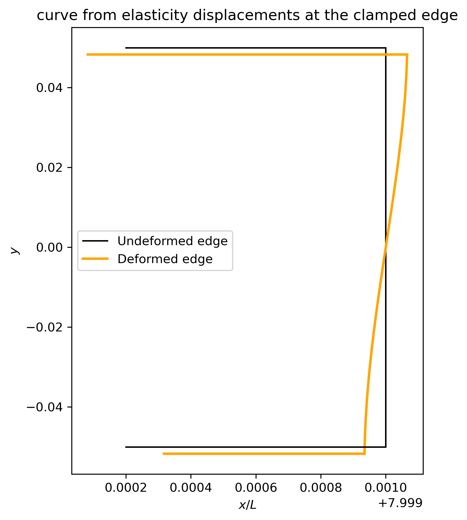
Distortion of the Cross Section
A key insight from the elasticity solution is that cross-sectional planes, initially flat and perpendicular to the neutral axis, do not remain planar after deformation when shear stresses are present. This behavior contrasts with the assumption of the Euler–Bernoulli beam theory, which presumes that “plane sections remain plane.” The figure below illustrates the resulting distortion of the end cross-section.