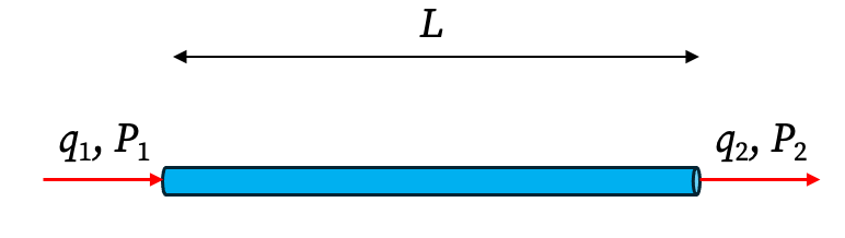
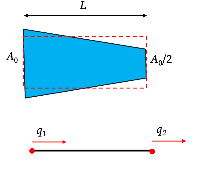
Let’s derive the well-known stiffness matrix for a simple two-node truss (bar) element. That is, we consider two degrees of freedom \(q_1\) and \(q_2\) at the two ends and their corresponding forces \(P_1\) and \(P_2\).
From Standard Matrix Analysis:
The equilibrium of the forces requires that \(P_1=-P_2\). From the strength of materials we know \[ \frac{P_1}{A}=E\frac{q_1-q_2}{L}, \qquad \frac{P_2}{A}=E\frac{q_2-q_1}{L}, \] The above equations can be written as \[ P_1=\frac{EA}{L}(q_1-q_2),P_2=\frac{EA}{L}(q_2-q_1) \]
From structural analysis, we know the stiffness matrix for a bar with constant cross-sectional area A, Young’s modulus E and length L is: \[ \mathbf{K} = \frac{EA}{L} \begin{bmatrix} 1 & -1 \\ -1 & 1 \end{bmatrix} \]
From FEM First Principles: Now, let’s derive this using the FEM integral \(\mathbf{K} = \int \mathbf{B}^{\mathsf T} \mathbf{E} \mathbf{B} dV\).
Displacement Field: The axial displacement
u(x)at any point along the bar can be interpolated from the nodal displacementsq₁andq₂using linear shape functions. If \(q_1=1\) and \(q_2=0\), then \[u(x)=1-\frac{x}{L}\] and if \(q_1=0\) and \(q_2=1\), then \[u(x)=\frac{x}{L}\]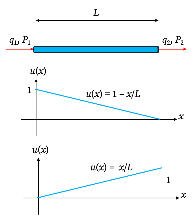
Using supperposition, we get \[ u(x) = \left(1 - \frac{x}{L}\right)q_1 + \left(\frac{x}{L}\right)q_2 = \mathbf{H}(x) \begin{bmatrix} q_1\\ q_2 \end{bmatrix} \] where \[\mathbf{H}=\begin{bmatrix} 1-\dfrac{x}{L} & \dfrac{x}{L}\end{bmatrix}\] is the shape function matrix.
- Strain Field: The axial strain
εis the derivative of the displacement. \[ \epsilon = \frac{du}{dx} = \frac{d\mathbf{H}}{dx} \mathbf{q} = \left[ -\frac{1}{L} \quad \frac{1}{L} \right] \begin{Bmatrix} q_1 \\ q_2 \end{Bmatrix} \] - Strain-Displacement Matrix (B): From the above, we see that for this simple element, the B matrix is constant: \[ \mathbf{B} = \left[ -\frac{1}{L} \quad \frac{1}{L} \right] \]
- Material Matrix (E): For 1D axial stress, the material matrix E is simply the scalar Young’s Modulus,
E. Integration: Now we compute the stiffness matrix integral over the element’s volume (
dV = A dx). \[ \mathbf{K} = \int_{0}^{L} \mathbf{B}^T E \mathbf{B} \,A \,dx \] \[ \begin{aligned} \mathbf{K} &= \int_{0}^{L} \begin{bmatrix} -1/L \\ 1/L \end{bmatrix} E \left[ -1/L \quad 1/L \right] A \,dx \\ &= E A \int_{0}^{L} \frac{1}{L^2} \begin{bmatrix} 1 & -1 \\ -1 & 1 \end{bmatrix} dx \end{aligned} \]Since everything inside the integral is constant with respect to
x: \[ \mathbf{K} = \frac{EA}{L^2} \begin{bmatrix} 1 & -1 \\ -1 & 1 \end{bmatrix} [x]_0^L = \frac{EA}{L} \begin{bmatrix} 1 & -1 \\ -1 & 1 \end{bmatrix} \]This successfully reproduces the known result using the fundamental principles of FEM.
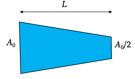
Analysis of a Tapered Bar
Consider a bar of length L that is fixed at one end and subjected to a point load P₁ at the other. Its cross-sectional area varies linearly: \[ A(x)=A_0\left(1-\frac{x}{2L}\right). \]
1. Analytical Solution
We can find the “exact” displacement by integrating the strain along the length.
Because there is no distributed force, the inter force at each point \[A(x) E\epsilon(x)=A(x) E \frac{du}{dx}\] must be a constant equal to the axial force \(P\). Therefore, \[A(x) E \frac{du}{dx}=P\] Therefore \[\int_0^L \frac{du}{dx} dx = \int_0^L \frac{P}{EA(x)} dx\]
But \[ \int_0^L \underbrace{\frac{du}{dx} dx}_{du}=u(L)-u(0)=q_2-q_1 \] and \[ \int_0^L \frac{P}{EA(x)} dx=\frac{P}{E}\int\frac{1}{1-\frac{x}{2L}}dx=\frac{P}{EA_0}L \ln 4 \] Since \(P=P_2=-P_1\), \[ \begin{bmatrix} P_1\\ P_2 \end{bmatrix}=\frac{EA_0}{L \ln 4}\begin{bmatrix} 1 & -1\\ -1 & 1 \end{bmatrix}\begin{bmatrix} q_1\\ q_2 \end{bmatrix} \] Thus the exact stiffness matrix is \[ \mathbf{K}=0.7213\frac{EA_0}{L}\begin{bmatrix} 1 & -1\\ -1 & 1 \end{bmatrix} \]
2. FEM Solution (Single Linear Element)
We now model the same bar with a single two-node finite element. We use the same linear shape functions as the truss example, which means our B matrix is again \[ \mathbf{B}=\frac{1}{L}\begin{bmatrix} 1 & -1 \end{bmatrix} \]
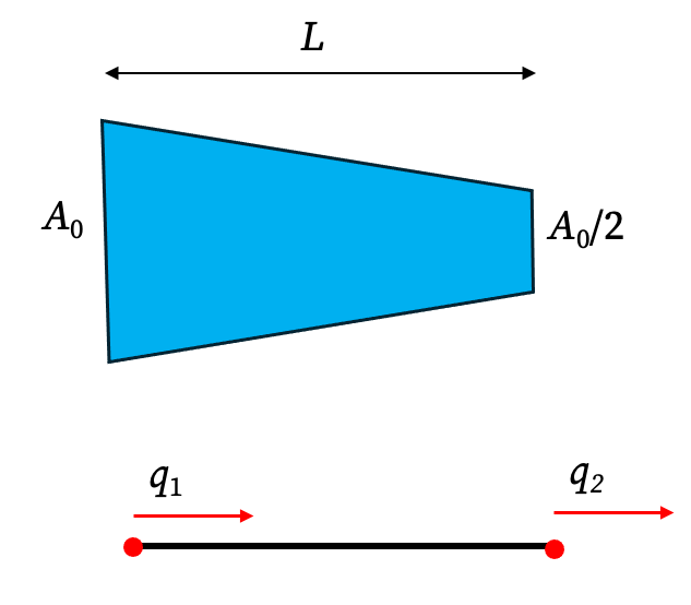
The key difference is that the area A(x) is now inside the stiffness integral:
\[ \mathbf{K} = \int_0^L \mathbf{B}^T E \mathbf{B} A(x) \,dx = \mathbf{B}^T E \mathbf{B} \int_0^L A(x) \,dx \]
\[ \int_0^L A(x) \,dx = \int_0^L A_0 \left(1 - \frac{x}{2L}\right) \,dx = A_0 \left[ x - \frac{x^2}{4L} \right]_0^L = 0.75 A_0 L \]
Substituting this back into the expression for K:
\[ \mathbf{K} = \left( \frac{E}{L^2} \begin{bmatrix} 1 & -1 \\ -1 & 1 \end{bmatrix} \right) (0.75 A_0 L) = \frac{0.75 E A_0}{L} \begin{bmatrix} 1 & -1 \\ -1 & 1 \end{bmatrix} \] This result is an approximation. The assumption of a linear displacement field (u(x) = Hq) results in a constant strain field (ε = Bq), which cannot represent the true, varying strain in the tapered bar. This discrepancy leads to an error (in this case, the element is overly stiff).
In this method, it seems that we have replaced the bar with a bar with constant cross sectional area equal to the average cross sectional area \(\frac{3}{4}A\). The error is approximately only 4%.
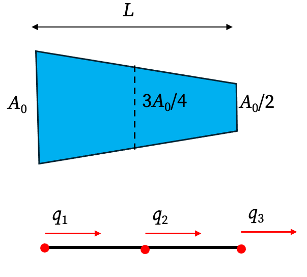
3. Improving FEM Accuracy: Two-Element Model of the Tapered Bar
Let’s model the tapered bar with two linear elements of length L/2. We can approximate the area as constant for each element, using the value at its midpoint.
- Element 1 (x = 0 to L/2): Midpoint at
x=L/4.A₁ = A₀(1 - (L/4)/2L) = (7/8)A₀. - Element 2 (x = L/2 to L): Midpoint at
x=3L/4.A₂ = A₀(1 - (3L/4)/2L) = (5/8)A₀.
The stiffness matrices are: \[ \mathbf{K}^{(1)} = \frac{E A_1}{L/2} \begin{bmatrix} 1 & -1 \\ -1 & 1 \end{bmatrix}_{1,2} \quad \mathbf{K}^{(2)} = \frac{E A_2}{L/2} \begin{bmatrix} 1 & -1 \\ -1 & 1 \end{bmatrix}_{2,3} \]
Assembly: We combine these into a 3x3 global stiffness matrix Kglobal by adding the contributions for each degree of freedom (node). \[ \mathbf{K}_{\rm global} = \frac{2E}{L} \begin{bmatrix} A_1 & -A_1 & 0 \\ -A_1 & A_1+A_2 & -A_2 \\ 0 & -A_2 & A_2 \end{bmatrix} \] \[ \mathbf{K}_{\rm global} = \frac{EA_0}{4} \begin{bmatrix} 7 & -7 & 0 \\ -7 & 7+5 & -5 \\ 0 & -5 & 5 \end{bmatrix} \]
Static Condensation:
Often, we are only interested in the relationship between the external degrees of freedom (nodes 1 and 3) and not the internal node (2). Static condensation is a matrix reduction technique used to eliminate internal d.o.f. The partitioned global system is: \[ \begin{Bmatrix} \mathbf{P}_e \\ \mathbf{P}_i \end{Bmatrix} = \begin{bmatrix} \mathbf{K}_{ee} & \mathbf{K}_{ei} \\ \mathbf{K}_{ie} & \mathbf{K}_{ii} \end{bmatrix} \begin{Bmatrix} \mathbf{q}_e \\ \mathbf{q}_i \end{Bmatrix} \] This can be written as \[ \mathbf{P}_e=\mathbf{K}_{ee} \mathbf{q}_e+\mathbf{K}_{ei}\mathbf{q}_i \] \[ \mathbf{P}_i=\mathbf{K}_{ie}\mathbf{q}_e+\mathbf{K}_{ii}\mathbf{q}_i \] If no forces are applied to the internal nodes (Pi = 0), we can solve for qi and substitute it back to find a condensed stiffness matrix Kcondensed relating only the external d.o.f. \[ \mathbf{0}=\mathbf{K}_{ie}\mathbf{q}_e+\mathbf{K}_{ii}\mathbf{q}_i \] \[ \mathbf{q}_i=-\mathbf{K}_{ii}^{-1}\mathbf{K}_{ie}\mathbf{q}_e \]
\[ \mathbf{K}_{\rm condensed} = \mathbf{K}_{ee} - \mathbf{K}_{ei} \mathbf{K}_{ii}^{-1} \mathbf{K}_{ie} \]
Applying this to our two-element model \[ \mathbf{K}_{ee}=\frac{EA_0}{4}\begin{bmatrix} 7 & 0\\ 0 & 5 \end{bmatrix},\quad \mathbf{K}_{ei}=\frac{EA_0}{4}\begin{bmatrix} -7 \\ -5 \end{bmatrix} \] \[ \mathbf{K}_{ei}=\frac{EA_0}{4}\begin{bmatrix} -7 & -5 \end{bmatrix}, \quad \mathbf{K}_{ii}=\frac{12 E A_0}{4} \] yields a 2x2 matrix \[ \mathbf{K}_{\rm condensed}=0.7229\frac{EA_0}{L}\begin{bmatrix} 1 & -1\\ -1 & 1 \end{bmatrix} \]
that provides a much more accurate result for the bar’s stiffness, significantly reducing the error (about 0.2%).
4.2. Higher-Order Elements
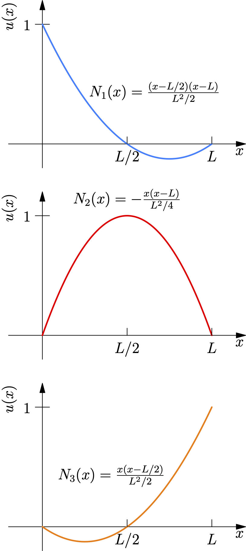
Instead of using more simple elements, we can use a single, more complex element. A quadratic element, for instance, has a third node at its midpoint and uses second-order polynomials for its shape functions.
For a 3-node bar element (nodes at x=0, L, L/2), the displacement field is: \[ u(x) =\begin{bmatrix}N_1(x) & N_2(x) & N_3(x)\end{bmatrix}\begin{bmatrix}q_1 \\ q_2 \\ q_3\end{bmatrix}\] where N₁, N₂, N₃ are quadratic functions: \[ N_1^{(2)}(x)=\frac{(x-L/2)(x-L)}{L^2/2}, \] \[ N_2^{(2)}(x)=-\frac{x(x-L)}{L^2/4}, \] \[ N_3^{(2)}(x)=\frac{x(x-L/2)}{L^2/2}. \]
This leads to a strain field ε(x) that varies linearly, which is a much better approximation for the tapered bar. \[ \epsilon=\frac{du}{dx}=\underbrace{\begin{bmatrix}\dfrac{dN_1}{dx} & \dfrac{dN_2}{dx} & \dfrac{dN_3}{dx}\end{bmatrix}}_{\mathbf{B}}\begin{bmatrix}q_1 \\ q_2 \\ q_3\end{bmatrix} \] Calculating the 3x3 stiffness matrix \[ \begin{aligned} \mathbf{K}_{3\times 3} &= \int_{0}^{L} \mathbf{B}^{\mathsf T}_{3\times 1}\,E\,\mathbf{B}_{1\times 3}\ \overbrace{A_0\left(1-\frac{x}{2L}\right) dx}^{dV} \\[9pt] &=\frac{EA_0}{L} \begin{bmatrix} \dfrac{25}{12} & -\dfrac{7}{3} & \dfrac{1}{4} \\ -\dfrac{7}{3} & 4 & -\dfrac{5}{3} \\ \dfrac{1}{4} & -\dfrac{5}{3} & \dfrac{17}{12} \end{bmatrix} . \end{aligned} \]
and then using static condensation to get a 2x2 external stiffness matrix results in a highly accurate solution (error of ~0.12% in the example): \[ \mathbf{K}^{\text{cond}}_{2\times 2} = \frac{13}{18}\frac{EA_0}{L} \begin{bmatrix} 1 & -1\\ -1 & 1 \end{bmatrix} \approx 0.7222\frac{EA_0}{L} \begin{bmatrix} 1 & -1\\ -1 & 1 \end{bmatrix}. \]
If we take shape functions linear
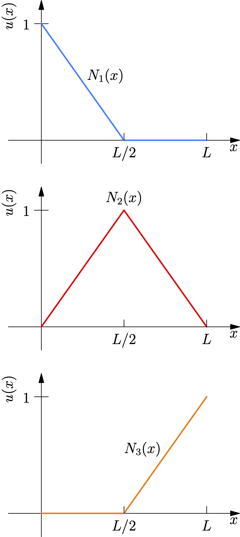
then the result will be identical to the case where we chose two elements.