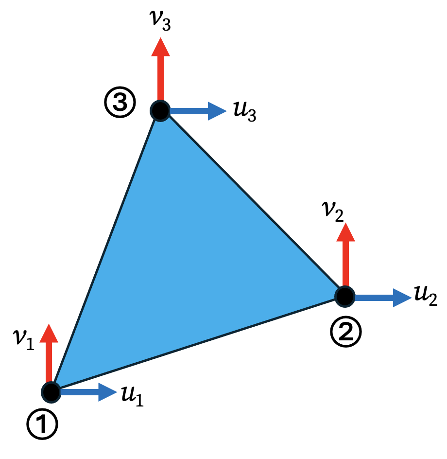
We now extend the principles of the Finite Element Method to two-dimensional domains. The simplest element for discretizing a 2D continuum is the Triangular Element. Let’s consider three nodes at each corner of the triangle and the nodes are numbered in counter clock wise order. Each node has two degrees of freedom \(u_i\) and \(v_i\).

1. Formulation for Two-Dimensional Elasticity

Before deriving the properties of this element, we must establish the governing relationships for two-dimensional elasticity.

The state of stress and strain at any point can be represented by vectors.

The Voigt stress vector is defined as: \[ \{\sigma\} = \begin{Bmatrix} \sigma_{xx} \\ \sigma_{yy} \\ \sigma_{xy} \end{Bmatrix} \]

The corresponding Voigt strain vector is: \[ \{\epsilon\} = \begin{Bmatrix} \epsilon_{xx} \\ \epsilon_{yy} \\ \gamma_{xy} \end{Bmatrix} \]

The relationship between stress and strain is the constitutive law, which for a linear elastic material is expressed in matrix form as: \[ \{\sigma\} = [E] \{\epsilon\} \] Here, E is the elasticity matrix, containing the material properties. (This matrix is not to be confused with the scalar Young’s Modulus, E, used in its definition).

For 2D problems, one of two simplifying assumptions is typically made: plane stress or plane strain.

Plane Stress: Assumed for thin structures loaded in their own plane (\(\sigma_{zz}=0\)). The elasticity matrix is: \[ \mathbf{E} = \frac{E}{1-\nu^2} \begin{bmatrix} 1 & \nu & 0 \\ \nu & 1 & 0 \\ 0 & 0 & \frac{1-\nu}{2} \end{bmatrix} \]

Plane Strain: Assumed for long structures with a uniform cross-section where out-of-plane strain is zero (\(\epsilon_{zz}=0\)). The elasticity matrix is: \[ \mathbf{E} = \frac{E(1-\nu)}{(1+\nu)(1-2\nu)} \begin{bmatrix} 1 & \frac{\nu}{1-\nu} & 0 \\ \frac{\nu}{1-\nu} & 1 & 0 \\ 0 & 0 & \frac{1-2\nu}{2(1-\nu)} \end{bmatrix} \]

2 The Strain-Displacement Matrix [B]

Assumptions: The displacement field within the element, u(x,y) in the x-direction and v(x,y) in the y-direction, is interpolated from the nodal displacement values using shape functions N_i. It is assumed that the displacement in a given direction depends only on the nodal displacements in that same direction. \[ u = \sum_{i=1}^3 N_i u_i \quad , \quad v = \sum_{i=1}^3 N_i v_i \]

The strains are the derivatives of the displacement field. For a two-dimensional problem, the relationships are:

\[ \epsilon_{xx} = \frac{\partial u}{\partial x} \quad, \quad \epsilon_{yy} = \frac{\partial v}{\partial y} \quad, \quad \epsilon_{xy} = \frac{\partial u}{\partial y} + \frac{\partial v}{\partial x} \]

By substituting the interpolated displacement fields into these strain definitions, we can construct a relationship between the Voigt strain vector \(\{\epsilon\}\) and the vector of nodal displacements \(\mathbf{q}\). This relationship defines the strain-displacement matrix, B.

\[ \{\epsilon\} = [B] \{q\} \]

For a 3-node triangular element, the nodal displacement vector is ordered as:

\[ \mathbf{q} = \begin{Bmatrix} u_1 \\ v_1 \\ u_2 \\ v_2 \\ u_3 \\ v_3 \end{Bmatrix} \]

The strain-displacement matrix B is therefore a \(3 \times 6\) matrix composed of the derivatives of the shape functions:

\[ \mathbf{B} = \begin{bmatrix} \frac{\partial N_1}{\partial x} & 0 & \frac{\partial N_2}{\partial x} & 0 & \frac{\partial N_3}{\partial x} & 0 \\ 0 & \frac{\partial N_1}{\partial y} & 0 & \frac{\partial N_2}{\partial y} & 0 & \frac{\partial N_3}{\partial y} \\ \frac{\partial N_1}{\partial y} & \frac{\partial N_1}{\partial x} & \frac{\partial N_2}{\partial y} & \frac{\partial N_2}{\partial x} & \frac{\partial N_3}{\partial y} & \frac{\partial N_3}{\partial x} \end{bmatrix} \]

3. Derivation of Shape Functions

To determine the B matrix, we must first find the explicit form of the shape functions, N_i. For the 3-node triangular element, we assume the simplest possible displacement field: a linear polynomial.

\[ \begin{aligned} u(x,y) &= A_1 + A_2 x + A_3 y\\ &=\langle 1 \quad x\quad y\rangle\begin{Bmatrix} A_1\\ A_2\\ A_3 \end{Bmatrix} \end{aligned} \]

The coefficients A₁, A₂, and A₃ are constants. To relate them to the physical nodal displacements, we enforce this equation at each of the three nodes:

\[ \begin{Bmatrix} u_1 \\ u_2 \\ u_3 \end{Bmatrix} = \begin{bmatrix} 1 & x_1 & y_1 \\ 1 & x_2 & y_2 \\ 1 & x_3 & y_3 \end{bmatrix} \begin{Bmatrix} A_1 \\ A_2 \\ A_3 \end{Bmatrix} \]

This system of equations can be inverted to solve for the coefficients A_i in terms of the nodal displacements u_i and the nodal coordinates.

\[ \begin{aligned} \begin{Bmatrix} A_1 \\ A_2 \\ A_3 \end{Bmatrix} &= \frac{1}{2A} \begin{bmatrix} x_2 y_3 - x_3 y_2 & x_3 y_1 - x_1 y_3 & x_1 y_2 - x_2 y_1 \\ y_2 - y_3 & y_3 - y_1 & y_1 - y_2 \\ x_3 - x_2 & x_1 - x_3 & x_2 - x_1 \end{bmatrix} \begin{Bmatrix} u_1 \\ u_2 \\ u_3 \end{Bmatrix}\\[9pt] &=\frac{1}{2A}\begin{bmatrix} a_1 & a_2 & a_3\\ b_1 & b_2 & b_3\\ c_1 & c_2 & c_3 \end{bmatrix}\begin{Bmatrix} u_1 \\ u_2 \\ u_3 \end{Bmatrix} \end{aligned}\] where \[ A = \frac{1}{2}\begin{vmatrix} 1 & x_1 & y_1\\ 1 & x_2 & y_2\\ 1 & x_3 & y_3 \end{vmatrix} \] is the area of the triangle.

Substituting these back into the linear polynomial and rearranging leads to the final form of the shape functions:

\[ \begin{aligned} u&=\langle 1 \quad x\quad y\rangle\begin{Bmatrix} A_1\\ A_2\\ A_3 \end{Bmatrix}\\ &=\langle 1 \quad x\quad y\rangle \frac{1}{2A}\begin{bmatrix} a_1 & a_2 & a_3\\ b_1 & b_2 & b_3\\ c_1 & c_2 & c_3 \end{bmatrix}\begin{Bmatrix} u_1 \\ u_2 \\ u_3 \end{Bmatrix}\\ &=\langle N_1\quad N_2 \quad N_3\rangle \begin{Bmatrix} u_1 \\ u_2 \\ u_3 \end{Bmatrix} \end{aligned} \]

The shape functions derived from the linear polynomial field take the form:

\[ N_i(x,y) = \frac{1}{2A}(a_i + b_i x + c_i y) \] where A is the area of the element and a_i, b_i, and c_i are coefficients composed of the nodal coordinates.

4. The Constant Strain B Matrix and Element Stiffness

The derivatives of these shape functions are: \[ \frac{\partial N_i}{\partial x} = \frac{b_i}{2A} \quad , \quad \frac{\partial N_i}{\partial y} = \frac{c_i}{2A} \]

A critical consequence of the linear shape function is that its derivatives are constant. Since the B matrix is composed entirely of these derivatives, the B matrix for this element is also constant. From the relation \(\{\epsilon\} = [B] \{q\}\), this implies that the strain ϵ is uniform throughout the element, which is why it is named the Constant Strain Triangle (CST).

The element stiffness matrix K is found by integrating over the element domain Ω: \[ \mathbf{K} = \int_{\Omega} \mathbf{B}^{\mathsf T}\mathbf{E}\ \mathbf{B} \, dV \]

For an element of constant thickness t, this volume integral becomes an area integral: \[\mathbf{K} = \int_{A} \mathbf{B}^{\mathsf T}\mathbf{E}\,\mathbf{B}\, t\, dA \]

Since B, E, and t are all constant, they can be taken outside the integral, which simplifies to the area A. This yields the final expression for the element stiffness matrix:

\[ \mathbf{K} = (\mathbf{B}^{\mathsf T}\mathbf{E}\,\mathbf{B}) t A \]

5. Inter-Element Continuity and Higher-Order Elements

A question arises regarding the continuity of displacement. We know displacement is continuous at the nodes, but is it continuous along the edges between nodes?

The answer is yes. Since the displacement field is linear, its variation along any edge is a linear interpolation between the two corner nodal values. An adjacent element sharing that edge will have its displacement field described by the exact same linear interpolation. This ensures displacement compatibility between elements, a condition known as \(C^0\) continuity.

The completeness condition, which ensures the element can represent rigid-body motion, is satisfied, as indicated by the property:

\[ \sum N_i = 1 \]

The accuracy of the CST element is limited by its constant strain assumption. To model problems with varying strain fields more accurately, higher-order elements are used. This is achieved by adding nodes to the element and using higher-order polynomials for the shape functions. For instance, adding mid-side nodes allows for a quadratic displacement field (a 6-node triangle), which results in a linearly varying strain field.

These higher-order elements still possess only \(C^0\) continuity. Achieving higher continuity (e.g., \(C^1\), where derivatives are also continuous) requires more complex element formulations.