1. Fundamental Concept

The Finite Element Method (FEM) is fundamentally an application of the Principle of Virtual Work. Let’s see what this principle states.

Virtual Displacement

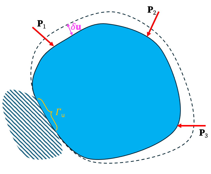
Consider a virtual displacement field \(\delta\mathbf{u}\) in the body. The virtual displacement is arbitrary¹ except that it must comply with the boundary constraints; that is, it is zero wherever the displacement is prescribed on the boundary.

External Virtual Work (EVW)

The external virtual work (EVW) is the work done by the real tractions and body forces and is given by \[ EVW =\int_{\Gamma_t} \mathbf{t}\cdot \delta\mathbf{u}\ dS+\int_\Omega \mathbf{b}\cdot \delta\mathbf{u}\ dV \] The first integral is over the portion of the boundary of the body (𝛤_t)where traction is prescribed. The second integral is over the volume (Ω) of the body.

If body forces are negligible and only concentrated forces P act at certain nodes (or if distributed tractions are converted to equivalent nodal forces, as will be explained later), then the external virtual work reduces to \[ VW_E = \delta\mathbf{q}^{\mathsf T} \mathbf{P} \] where:

• P is the vector of real external loads (forces) applied to the structure’s nodes.
• \(\delta\mathbf{q}\) is the vector of virtual external displacements at the corresponding nodes.

Internal Virtual Work (IVW)

The internal virtual work is the integral of the product of the real internal stress, σ, and the virtual strain, \(\delta\boldsymbol{\epsilon}\), over the volume (Ω) of the body.

\[ IVW= \int_{\Omega} \delta\boldsymbol{\epsilon}^{\mathsf T} \boldsymbol{\sigma} \,dV \] where:

• \(\delta\boldsymbol{\epsilon}\) is the virtual strain resulting from the virtual displacement \(\delta\mathbf{u}\). \[ \delta\boldsymbol{\epsilon}=\begin{bmatrix} \delta\epsilon_{xx} \\ \delta\epsilon_{yy} \\ \delta\epsilon_{zz} \\ \delta\gamma_{zx}\\ \delta\gamma_{zy}\\ \delta\gamma_{xy} \end{bmatrix} \]
• σ is the real internal stress resulting from the real external load P. \[ \boldsymbol{\sigma}=\begin{bmatrix} \sigma_{xx} \\ \sigma_{yy} \\ \sigma_{zz} \\ \sigma_{zx}\\ \sigma_{zy}\\ \sigma_{xy} \end{bmatrix} \]

If the material is linear elastic, then using the constitutive relationship (Hooke’s Law for a linear elastic material), we can express stress in terms of strain:

\[ \bbox[5px,border:1px #f2f2f2;background-color:#f2f2f2]{\boldsymbol{\sigma} = \mathbf{E} \boldsymbol{\epsilon}} \]

• ε is the real strain corresponding to the real stress σ.
• E is the material elasticity matrix (containing properties like Young’s Modulus and Poisson’s Ratio). For example, in a plane strain problem: \[ \mathbf{E} = \frac{E}{(1+\nu)(1-2\nu)} \begin{bmatrix} 1-\nu & \nu & 0 \\ \nu & 1-\nu & 0 \\ 0 & 0 & \frac{1-2\nu}{2} \end{bmatrix}\] Substituting the constitutive law into the IVW expression gives: \[ IVW = \int_{\Omega} \delta\boldsymbol{\epsilon}^{\mathsf T} \mathbf{E} \boldsymbol{\epsilon} \,dV \]

Principle of Virtual Work

The principle of virtual work states that the body is in equilibrium if and only the external virtual work (EVM) is equal to the internal virtual work (IVE) for every admissible virtual displacement field. \[ EVW=IVW \] or \[ \delta\mathbf{q}^T\mathbf{P}=\int_\Omega\delta\boldsymbol{\epsilon}^{\mathsf T}\boldsymbol{\sigma}\ dV \] We previously proved this principle.

2. The Strain-Displacement Matrix (B)

A core concept in FEM is relating the continuous strain field within an element to its discrete nodal displacements, q. This is achieved through the strain-displacement matrix, B. \[ \bbox[5px,border:1px #f2f2f2;background-color:#f2f2f2]{\boldsymbol{\epsilon}=\mathbf{B}\mathbf{q}} \]

The B matrix is derived from the derivatives of the element’s shape functions, which will be discussed later, and is, in the general case, a function of the coordinates x = (x, y, z) within the element. For emphasize, we may write: \[ \boldsymbol{\epsilon}(\mathbf{x}) = \mathbf{B}(\mathbf{x}) \mathbf{q} \]

Similarly, the virtual strain is related to the virtual nodal displacements:

\[ \delta\boldsymbol{\epsilon}(\mathbf{x}) = \mathbf{B}(\mathbf{x}) \delta\mathbf{q} \]

By substituting these relationships into the IVW equation, we can express the internal virtual work entirely in terms of nodal displacements: \[ \begin{aligned} IVW&= \int_{\Omega} \delta\boldsymbol{\epsilon}^{\mathsf T} \mathbf{E} \boldsymbol{\epsilon} \,d\Omega \\ &=\int_{\Omega} (\mathbf{B}\delta\mathbf{q})^{\mathsf T} \mathbf{E} (\mathbf{B}\mathbf{q}) \,d\Omega \\ &= \int_{\Omega} \delta\mathbf{q}^{\mathsf T} \mathbf{B}^{\mathsf T} \mathbf{E} \mathbf{B} \mathbf{q} \,d\Omega\\ &=\delta\mathbf{q}^{\mathsf T} \left(\int_{\Omega} \mathbf{B}^{\mathsf T} \mathbf{E} \mathbf{B} \,d\Omega\right) \mathbf{q} \end{aligned} \]

3. Derivation of the Element Stiffness Matrix (K)

By equating the expressions for external and internal virtual work:

\[ \delta\mathbf{q}^{\mathsf T} \mathbf{P} = \delta\mathbf{q}^{\mathsf T} \left( \int_{\Omega} \mathbf{B}^{\mathsf T} \mathbf{E} \mathbf{B} \,dV \right) \mathbf{q} \]

Since this equation must hold for any arbitrary virtual displacement \(\delta\mathbf{q}\), we can cancel the \(\delta\mathbf{q}^T\) term from both sides, yielding the fundamental relationship for a finite element:

\[ \bbox[5px,border:1px #f2f2f2;background-color:#f2f2f2]{\mathbf{P} = \mathbf{K} \mathbf{q}}\] where K is a square matrix called the stiffness matrix, defined as:

\[\bbox[5px,border:1px #f2f2f2;background-color:#f2f2f2]{ \mathbf{K} = \int_{\Omega} \mathbf{B}^{\mathsf T} \mathbf{E} \mathbf{B} \,dV }\]

This integral is the heart of the finite element formulation for linear static problems. It transforms the geometric and material properties into a matrix that relates nodal forces to nodal displacements.