The simple \[\frac{EA}{L} \begin{bmatrix} 1 & -1\\ -1& 1 \end{bmatrix} \]stiffness matrix (assuming constant cross sectional area and Young’s modulus) is only valid for a truss element aligned with a coordinate axis. In real structures, truss elements can be oriented at any angle. To handle this, we must derive a stiffness matrix that relates forces and displacements in a common global coordinate system (x, y).

The procedure is as follows: 1. Start with the simple stiffness matrix in a local coordinate system (x', y') that is aligned with the element. 2. Develop a transformation matrix, T, that relates the local and global coordinate systems. 3. Use this transformation matrix to convert the local stiffness matrix into the desired global stiffness matrix.
The Local Stiffness Matrix (Klocal)
For a truss element aligned with its local x' axis, it can only resist forces and experience displacements along that axis. Any force or displacement perpendicular to the element (in the y' direction) is associated with zero stiffness because it causes no change in length.
Therefore, we can write the stiffness matrix for the element in its local 2D coordinate system, which has four degrees of freedom (u₁', v₁', u₂', v₂'), as: \[ \begin{bmatrix} F_{x'}^{(1)} \\ F_{y'}^{(1)} \\ F_{x'}^{(2)} \\ F_{y'}^{(2)} \end{bmatrix} = \frac{EA}{L} \begin{bmatrix} 1 & 0 & -1 & 0 \\ 0 & 0 & 0 & 0 \\ -1 & 0 & 1 & 0 \\ 0 & 0 & 0 & 0 \end{bmatrix} \begin{bmatrix} u_{1'} \\ v_{1'} \\ u_{2'} \\ v_{2'} \end{bmatrix} \]
This 4x4 matrix is the stiffness matrix in local coordinate system, Klocal.

Coordinate Transformation
Let the global coordinate system (x, y) be rotated by an angle θ relative to the local system (x', y').
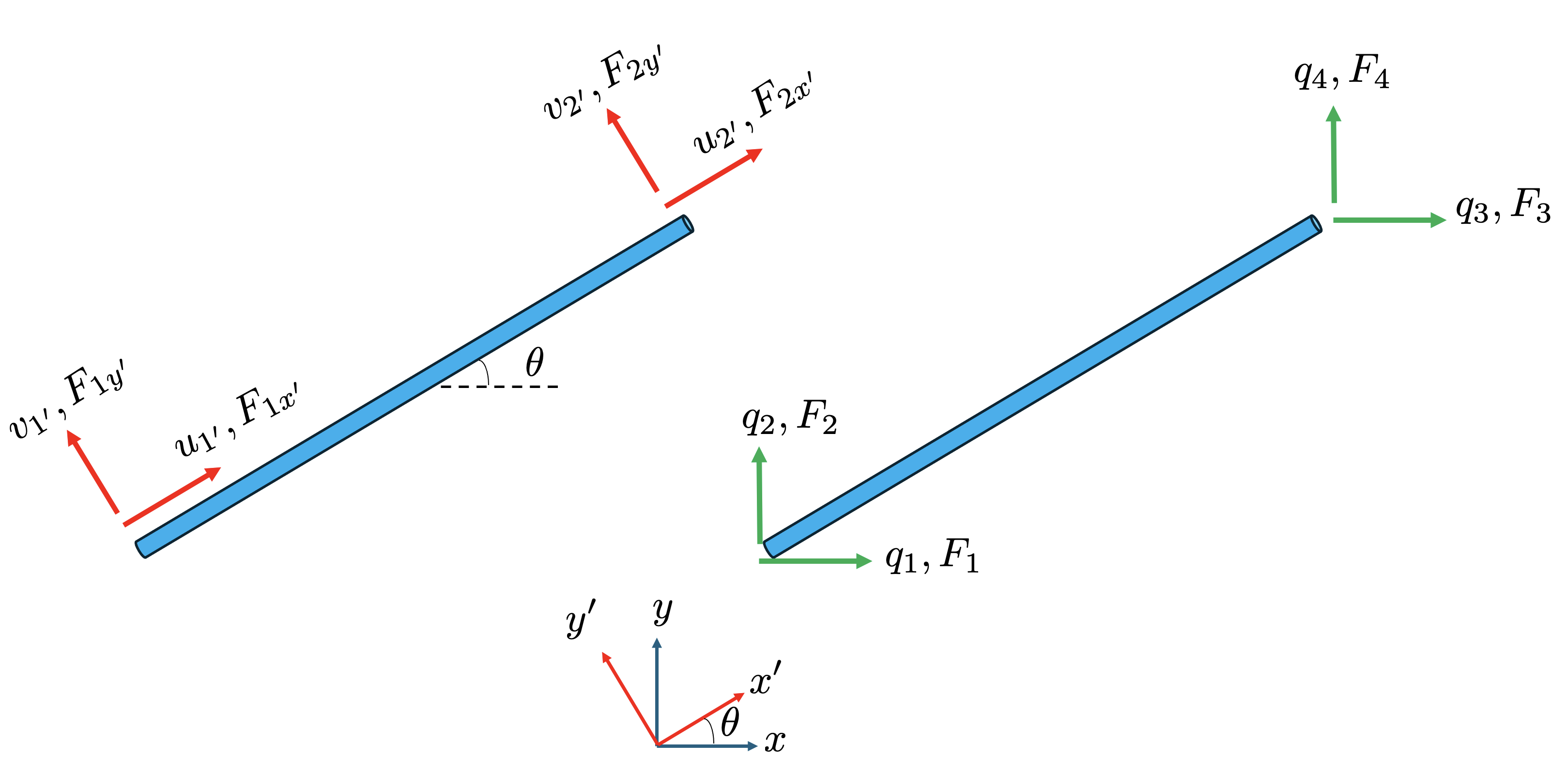
Any vector \(\mathbf{V}\) can be transformed from one system to the other using a standard 2D rotation matrix. The relationship between the local vector components [Vx’, Vy’] and the global components [Vx, Vy] is: \[ \begin{bmatrix} V_{x'} & V_{y'} \end{bmatrix}=\begin{bmatrix} V_{x} & V_{y} \end{bmatrix}\begin{bmatrix} \cos \theta & -\sin\theta\\ \sin\theta & \cos\theta \end{bmatrix} \] Taking the transpose of both sides give \[ \begin{bmatrix} V_{x'} \\ V_{y'} \end{bmatrix} = \begin{bmatrix} \cos\theta & \sin\theta \\ -\sin\theta & \cos\theta \end{bmatrix} \begin{bmatrix} V_x \\ V_y \end{bmatrix} \] Let c = cos(θ) and s = sin(θ). The rotation matrix is \[ \mathbf{R}=\begin{bmatrix} c & s\\ -s & c \end{bmatrix} \] We can apply this to the displacement vectors at each node. Let the global displacements be q and the local displacements be u’:
- At Node 1: \[ \begin{bmatrix}u_{1'} \\ v_{1'}\end{bmatrix} = \mathbf{R}\begin{bmatrix}q_{1} \\ q_{2}\end{bmatrix} \]
- At Node 2: \[ \begin{bmatrix}u_{2'} \\ v_{2'}\end{bmatrix} = \mathbf{R}\begin{bmatrix}q_{3} \\ q_{4}\end{bmatrix} \]
We can combine these into a single transformation for the entire element. This defines the transformation matrix, T:
\[ \begin{bmatrix} u_{1'} \\ v_{1'} \\ u_{2'} \\ v_{2'} \end{bmatrix} = \begin{bmatrix} c & s & 0 & 0 \\ -s & c & 0 & 0 \\ 0 & 0 & c & s \\ 0 & 0 & -s & c \end{bmatrix} \begin{bmatrix} q_1 \\ q_2 \\ q_3 \\ q_4 \end{bmatrix} \implies \mathbf{u'} = \mathbf{Tq} \]
A similar relationship exists for the force vectors: \[\mathbf{F}'=\mathbf{T}\mathbf{F}\] where F is the nodal force vector in the global xy coordinate system and F’ is the nodal force vector in the local x’y’ coordinate system.
Since T is an orthonormal matrix, its inverse is equal to its transpose T-1 = TT. Therefore, it follows from the above equation that: \[ \mathbf{F} = \mathbf{T}^{\mathsf T} \mathbf{F'} \] where #### Deriving the Global Stiffness Matrix (Kglobal)
We can now derive the stiffness matrix in the global coordinate system by combining these relationships:
- Start with the fundamental relationship in the local system: \[ \mathbf{F'} = \mathbf{K}^{\text{local}} \mathbf{u'} \]
- Substitute the displacement transformation u’ = Tq: \[ \mathbf{F'} = \mathbf{K}^{\text{local}} \mathbf{Tq} \]
- Pre-multiply both sides by TT to get the global forces F: \[ \mathbf{T}^{\mathsf T} \mathbf{F'} = \mathbf{T}^{\mathsf T} \mathbf{K}^{\text{local}} \mathbf{Tq} \]
- Recognize that the left side is the global force vector, F = **TTF’: \[ \mathbf{F} = \left( \mathbf{T}^{\mathsf T} \mathbf{K}^{\text{local}} \mathbf{T} \right) \mathbf{q} \]
This equation is now in the global form F = Kglobalq. Therefore, we have proven the master transformation equation for stiffness matrices:
\[ \bbox[5px,border:1px #f2f2f2;background-color:#f2f2f2]{ \mathbf{K}^{\text{global}} = \mathbf{T}^{\mathsf T} \mathbf{K}^{\text{local}} \mathbf{T} } \]
By carrying out this matrix multiplication, we arrive at the explicit form of the global stiffness matrix for an arbitrarily oriented truss element:
\[ \mathbf{K}^{\text{global}} = \frac{EA}{L} \begin{bmatrix} c^2 & cs & -c^2 & -cs \\ cs & s^2 & -cs & -s^2 \\ -c^2 & -cs & c^2 & cs \\ -cs & -s^2 & cs & s^2 \end{bmatrix} \]
This 4x4 matrix can now be used in the direct superposition (assembly) process described in the first section to build the global stiffness matrix for an entire truss structure.
The following example walks through the complete process of coordinate transformation and stiffness assembly.
Example: Analysis of a Three-Bar Truss Structure
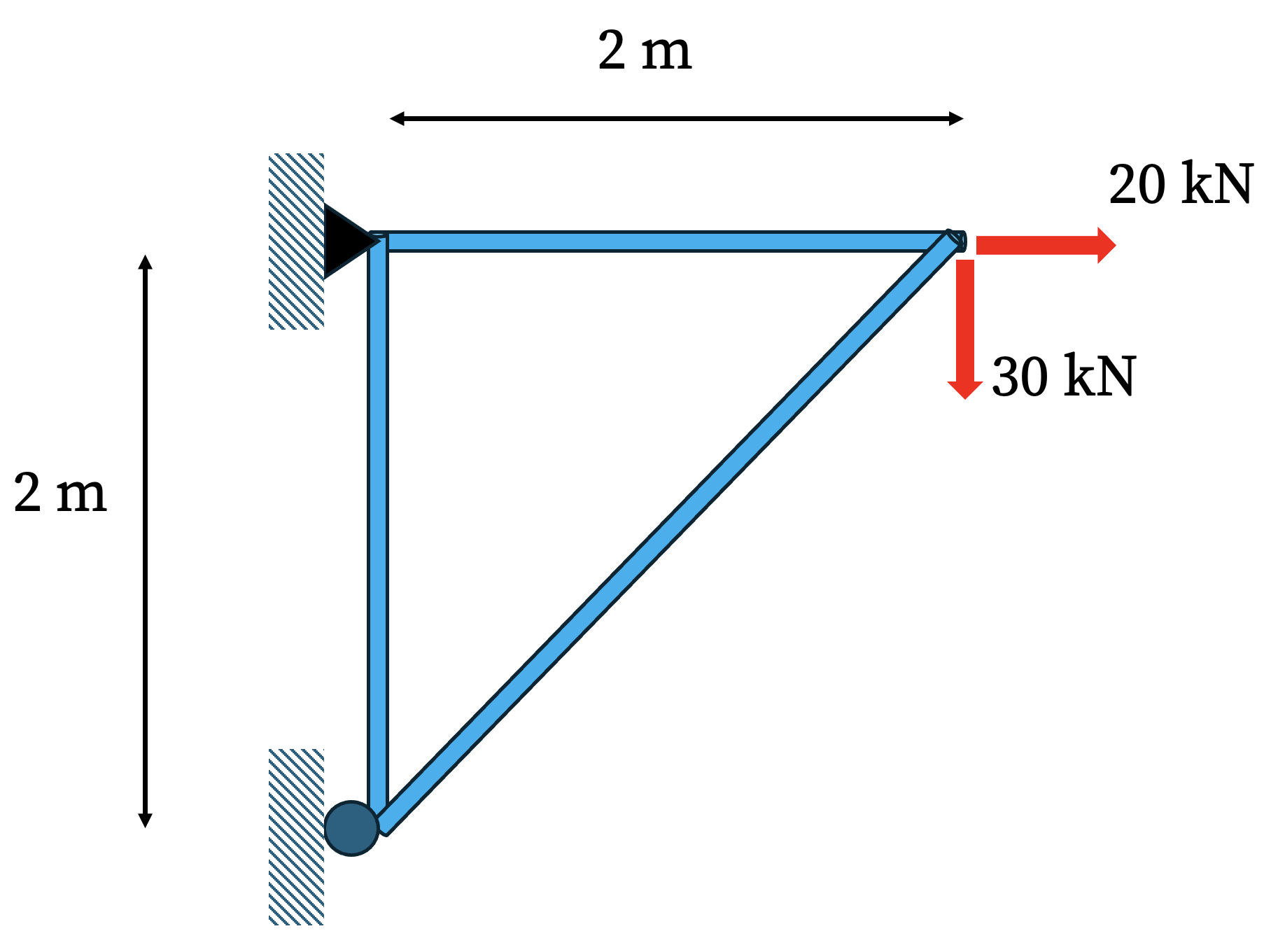
Let’s consider the following truss that withstand a horizontal and a vertical force (see the figure). Assume that Young’s modulus and cross-sectional area for all members is the same: E = 100 GPa, A = 200 mm2.
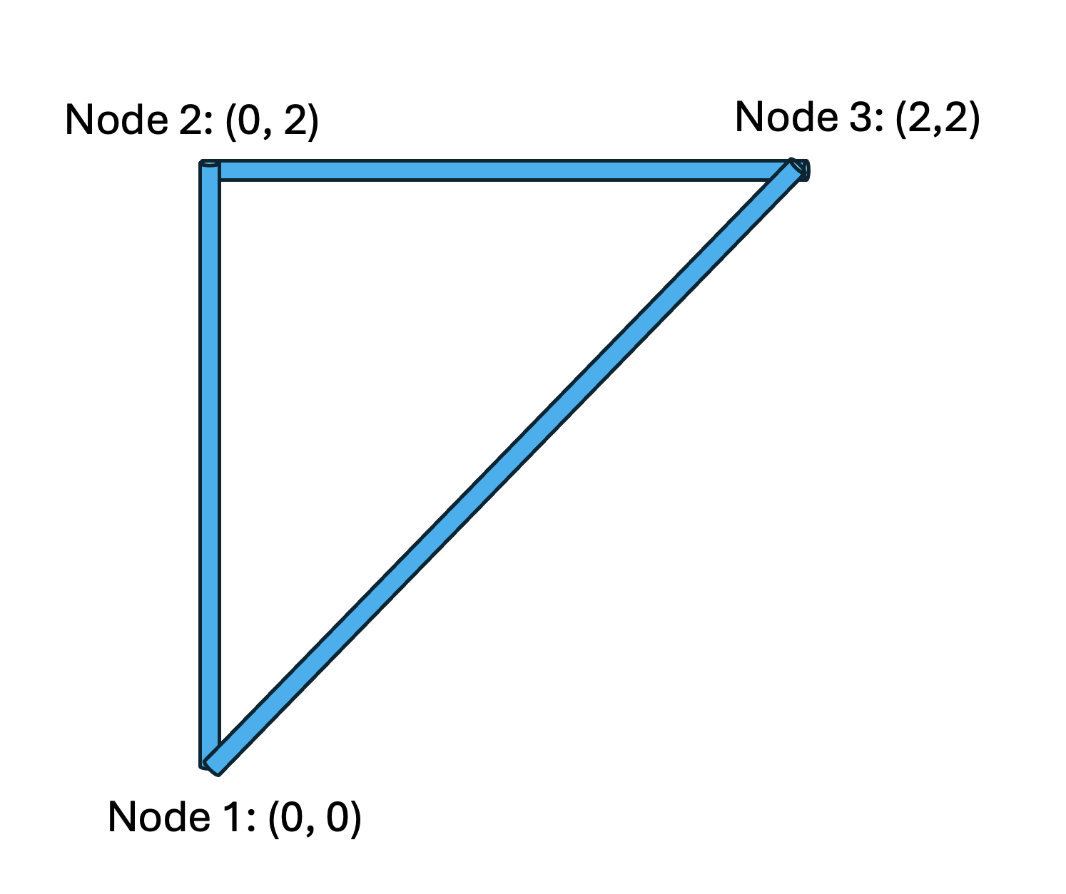
Global Coordinate System and Nodes: We establish a global \((x, y)\) coordinate system with the origin at node 1.
- Node 1: (0, 0)
- Node 2: (0, 2)
- Node 3: (2, 2)
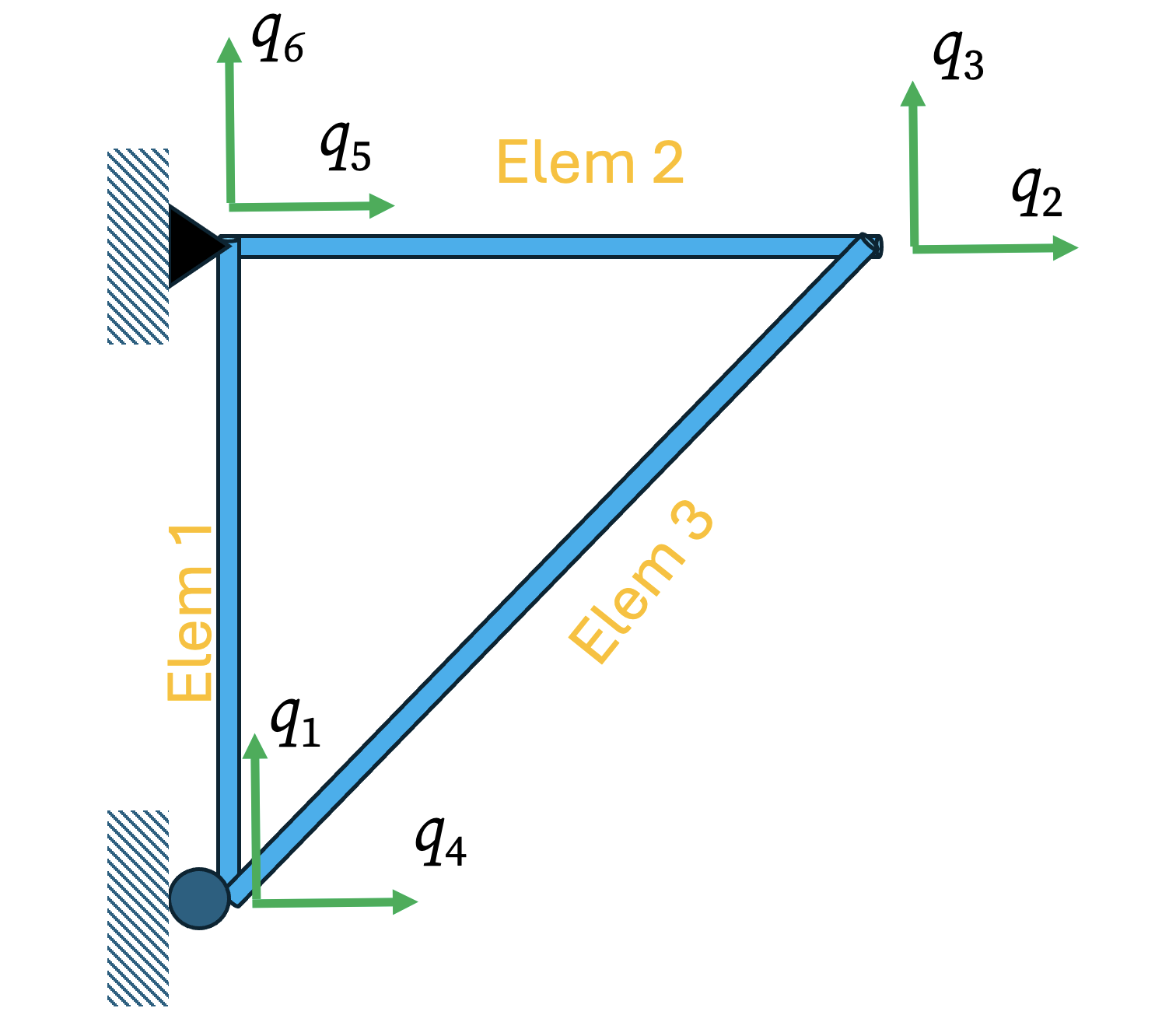
Global Degrees of Freedom (DOFs): The structure has 3 nodes, with 2 DOFs per node (\(u, v\)), for a total of 6 global DOFs. Let’s number the free DOFs first, followed by the supported (constrained) DOFs. This will simplify our calculations in the following.
- Free DOFs (at Node 3):
- \(q_1\): Vertical displacement at node 1
- \(q_2\): Horizontal displacement at node 3
- \(q_3\): Vertical displacement at node 3
- Supported DOFs (at Nodes 1 & 2):
- \(q_4\): Horizontal displacement at node 1
- \(q_5\): Horizontal displacement at node 2
- \(q_6\): Vertical displacement at node 2
Because nodes 1 is on a roller and node 2 is pinned, their corresponding displacements must be zero: \[ q_4 = q_5 = q_6 = 0 \]
Step 2: Deriving Each Element Stiffness Matrix in Global Coordinates
Now, we analyze each of the three truss elements individually, calculating its 4x4 stiffness matrix in the global coordinate system and explicitly labeling the rows and columns with the corresponding global DOF numbers.
Element ① (Nodes 1 to 2): * Length: \(L_1 = 2 \text{ m}\) * Angle: The element is vertical, so \(\theta = 90^\circ\). * Cosines: \(c = \cos(90^\circ) = 0\), \(s = \sin(90^\circ) = 1\). * DOF Mapping: The local DOFs for this element (\(u_1, v_1, u_2, v_2\)) correspond to the global DOFs (\(q_4, q_1, q_5, q_6\)). * Stiffness Matrix: \[ \begin{array}{cc} & \begin{array}{cccc} q_4 & q_1 &q_5 & q_6 \end{array} \\ \mathbf{K}_e^{(1)} = \dfrac{EA}{L} & \left[ \begin{array}{cccc} 0 & 0 & 0 & 0 \\ 0 & 1 & 0 & -1 \\ 0 & 0 & 0 & 0 \\ 0 & -1 & 0 & 1 \end{array} \right] \end{array} \begin{array}{c} \\ q_4 \\ q_1 \\ q_5 \\ q_6 \end{array} \]
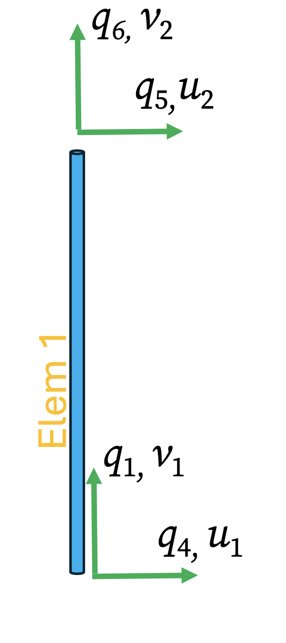
Element ② (Nodes 2 to 3):
- Length: \(L_2 = 2 \text{ m}\)
- Angle: The element is horizontal, so \(\theta = 0^\circ\).
- Cosines: \(c = \cos(0^\circ) = 1\), \(s = \sin(0^\circ) = 0\).
- DOF Mapping: The local DOFs for this element (\(u_2, v_2, u_3, v_3\)) correspond to the global DOFs (\(q_5, q_6, q_2, q_3\)).
- Stiffness Matrix: \[ \begin{array}{cc} & \begin{array}{cccc} q_5 & q_6 & q_2 & q_3 \end{array} \\ \mathbf{K}_e^{(2)} = \dfrac{EA}{L} & \left[ \begin{array}{cccc} 1 & 0 & -1 & 0 \\ 0 & 0 & 0 & 0 \\ -1 & 0 & 1 & 0 \\ 0 & 0 & 0 & 0 \end{array} \right] \end{array} \begin{array}{c} \\ q_5 \\ q_6 \\ q_2 \\ q_3 \end{array} \]
Element ③ (Nodes 1 to 3): * Length: \(L_3 = \sqrt{(2-0)^2 + (2-0)^2} = 2\sqrt{2} \text{ m}\) * Angle: The element is at 45°, so \(\theta = 45^\circ\). * Cosines: \(c = \cos(45^\circ) = 1/\sqrt{2}\), \(s = \sin(45^\circ) = 1/\sqrt{2}\). * DOF Mapping: The local DOFs for this element (\(u_1, v_1, u_3, v_3\)) correspond to the global DOFs (\(q_4, q_1, q_2, q_3\)). * Stiffness Matrix: For this element, \(c^2 = 1/2\), \(s^2 = 1/2\), \(cs = 1/2\). \[ \begin{array}{cc} & \begin{array}{cccc} q_4 & q_1 & q_2 & q_3 \end{array} \\ \mathbf{K}_e^{(3)} = \dfrac{EA}{2\sqrt{2} L} & \left[ \begin{array}{cccc} 1 & 1 & -1 & -1 \\ 1 & 1 & -1 & -1 \\ -1 & -1 & 1 & 1 \\ -1 & -1 & 1 & 1 \end{array} \right] \end{array} \begin{array}{c} \\q_4 \\ q_1 \\ q_2 \\ q_3 \end{array} \]
Step 3: Assembly of the Global Stiffness Matrix (\(\mathbf{K}\))
We now assemble the 6x6 global stiffness matrix by adding the components of each element matrix into the correct locations, guided by the global DOF labels. The final matrix \(\mathbf{K}\) is the sum of the three element stiffness matrices expanded into the 6x6 global space.
For example, let’s find the global term \(K_{11}\), which corresponds to the interaction between global DOFs \(q_1\) and \(q_1\). We look for the (q₁, q₁) entry in each element matrix:
- Element ①: The entry at row and column is \(\frac{EA}{L}\).
- Element ②: Does not have a row or column. Its contribution to \(K_{11}\) is 0.
- Element ③: The entry at row \(q_1\) and column \(q_1\) is \(\frac{EA}{2\sqrt{2}L}\).
- Total: \(K_{11} = \frac{EA}{L} + 0 + \frac{EA}{2\sqrt{2}L} = EA \left(\frac{1}{2} + \frac{1}{4\sqrt{2}}\right)\).
As another example, let’s find the off-diagonal term \(K_{16}\) (row 1, column 6): * Element ①: The entry at row \(q_1\) and column \(q_6\) is \(\frac{-EA}{L}\). * Element ②: Does not have a \(q_6\) and \(q_1\) DOF. Contribution is 0. * Element ③: Does not have a \(q_6\) and \(q_1\) DOF. Contribution is 0. * Total: \(K_{16} = - \frac{EA}{L} + 0 + 0 = -\frac{EA}{L}\).
This process of adding values based on their global row and column indices (direct superposition) is repeated for all 36 entries of the global stiffness matrix.
Step 4: Partitioning and Solving the System
The full system is \(\mathbf{P} = \mathbf{Kq}\). This assembled 6x6 \(\mathbf{K}\) matrix is singular because we have not yet applied the support conditions. We solve the system by partitioning it into free and supported DOFs.
\[ \begin{bmatrix} \mathbf{P}_f \\ \mathbf{P}_s \end{bmatrix} = \begin{bmatrix} \mathbf{K}_{ff} & \mathbf{K}_{fs} \\ \mathbf{K}_{sf} & \mathbf{K}_{ss} \end{bmatrix} \begin{bmatrix} \mathbf{q}_f \\ \mathbf{q}_s \end{bmatrix} \]
Where the partitions are: * Free Displacements: \(\mathbf{q}_f = \begin{bmatrix} q_1 \\ q_2 \\ q3\end{bmatrix}\) (These are the unknowns). * Support Displacements: \(\mathbf{q}_s = \begin{bmatrix} q_4 \\ q_5 \\ q_6 \end{bmatrix} = \mathbf{0}\). * Applied Forces: \(\mathbf{P}_f = \begin{bmatrix} P_1 \\ P_2 \\ P_3 \end{bmatrix} = \begin{bmatrix} 0 \\ 20000 \\ -30000 \end{bmatrix}\). * Support Reactions: \(\mathbf{P}_s = \begin{bmatrix} P_4 \\ P_5 \\ P_6 \end{bmatrix}\) (These are also unknown).
This single partitioned equation expands into two separate matrix equations: 1. \(\mathbf{P}_f = \mathbf{K}_{ff} \mathbf{q}_f + \mathbf{K}_{fs} \mathbf{q}_s\) 2. \(\mathbf{P}_s = \mathbf{K}_{sf} \mathbf{q}_f + \mathbf{K}_{ss} \mathbf{q}_s\)
Solving for the Unknown Displacements We apply the known boundary condition \(\mathbf{q}_s = \mathbf{0}\). This greatly simplifies the first equation: \[ \mathbf{P}_f = \mathbf{K}_{ff} \mathbf{q}_f + \mathbf{K}_{fs} (\mathbf{0}) \implies \mathbf{P}_f = \mathbf{K}_{ff} \mathbf{q}_f \] The matrix \(\mathbf{K}_{ff}\) is the top-left 3x3 partition of the global \(\mathbf{K}\) matrix, corresponding to the free DOFs \(q_1\), \(q_2\), and \(q_3\). We can now solve for the unknown displacements \(\mathbf{q}_f\) by inverting 1 this small, non-singular matrix: \[ \mathbf{q}_f = \mathbf{K}_{ff}^{-1} \mathbf{P}_f \] This calculation yields the numerical values for the horizontal and vertical displacements at node 3.
Solving for the Support Reactions Once the displacement vector \(\mathbf{q}_f\) is known, we can use the second equation (again with \(\mathbf{q}_s = \mathbf{0}\)) to find the unknown support reaction forces: \[ \mathbf{P}_s = \mathbf{K}_{sf} \mathbf{q}_f + \mathbf{K}_{ss} (\mathbf{0}) \implies \mathbf{P}_s = \mathbf{K}_{sf} \mathbf{q}_f \] This final step is a simple matrix-vector multiplication that gives the four reaction forces at the supports (nodes 1 and 2). This completes the analysis of the truss.
The following code, shows all the computations. It shows that \[ \mathbf{P}_s=\begin{bmatrix} 30\\ -50\\ 30 \end{bmatrix}~{\rm kN}. \]
- There are better and computationally cheaper ways to solve for \(\mathbf{P}_f\) than inverting \(\mathbf{K}_{ff}\).↩︎