While the triangular element is simple and can be used to mesh any two-dimensional geometry, its accuracy is limited by the assumption of constant strain. To improve upon this, we introduce the 4-node rectangular element. This element allows for a more complex strain distribution, leading to more accurate results.
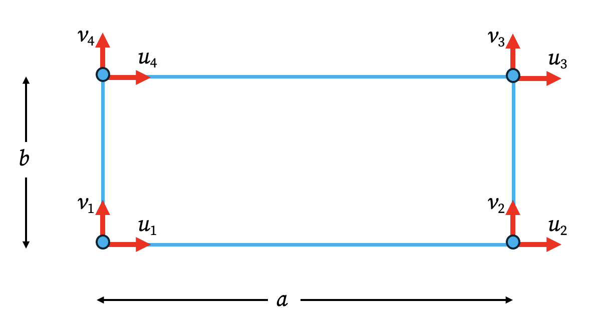
1. Displacement Field
For this element, the displacement field (e.g., for the u-displacement) is approximated using a four-term polynomial. A crucial addition is the xy term, which allows for a non-constant strain distribution.
\[ u(x,y) = a_1 + a_2x + a_3y + a_4xy \]
This can be written in matrix form: \[ u = \begin{Bmatrix} 1 & x & y & xy \end{Bmatrix} \begin{Bmatrix} a_1 \\ a_2 \\ a_3 \\ a_4 \end{Bmatrix} \]
By enforcing this equation at each of the four nodes, we can solve for the coefficients a in terms of the nodal displacements u. This leads to the familiar relationship \(u = \mathbf{N}\mathbf{u}\), where N is the vector of shape functions.
2. Shape Functions
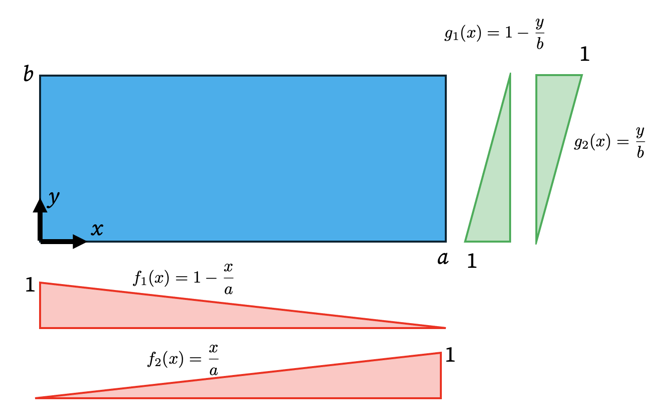
Instead of a brute-force matrix inversion, the shape functions for a rectangular element can be constructed elegantly through the product of one-dimensional linear interpolation functions. Consider a rectangle with dimensions a and b. We can define simple linear functions in each direction:
- In the x-direction: \(f_1(x) = 1 - \frac{x}{a}\) \(f_2(x) = \frac{x}{a}\)
- In the y-direction: \(g_1(y) = 1 - \frac{y}{b}\) \(g_2(y) = \frac{y}{b}\)
The two-dimensional shape functions are then formed by taking products of these 1D functions. For a node i, the shape function is the product of the 1D functions that are equal to 1 at that node.
- \(N_1(x,y) = f_1(x) g_1(y) = (1 - \frac{x}{a})(1 - \frac{y}{b})\)
- \(N_2(x,y) = f_2(x) g_1(y) = (\frac{x}{a})(1 - \frac{y}{b})\)
- \(N_3(x,y) = f_2(x) g_2(y) = (\frac{x}{a})(\frac{y}{b})\)
- \(N_4(x,y) = f_1(x) g_2(y) = (1 - \frac{x}{a})(\frac{y}{b})\)
3. Strain-Displacement Matrix and Stiffness
Since the shape functions now contain x and y terms, their derivatives are no longer constant. For example, for \(N_1\):
\[ \frac{\partial N_1}{\partial x} = -\frac{1}{a}\left(1-\frac{y}{b}\right) \quad , \quad \frac{\partial N_1}{\partial y} = -\frac{1}{b}\left(1-\frac{x}{a}\right) \]
The B matrix will now contain terms that are functions of x and y. This means that the strain, given by \(\{\epsilon\} = \mathbf{B}\mathbf{q}\), is no longer constant within the element. It can vary linearly, which is a significant improvement over the Constant Strain Triangle.
The element stiffness matrix is calculated using the standard formula:
\[ \mathbf{K} = \int_V \mathbf{B}^T \mathbf{E} \mathbf{B} \, dV = t \int_0^b \int_0^a \mathbf{B}(x,y)^T \mathbf{E} \mathbf{B}(x,y) \, dx dy \]
Because the B matrix is a function of x and y, the integrand is no longer a constant and the integration must be performed explicitly.