Beam elements are fundamental components in structural analysis, designed to model members that resist loads primarily through bending. Unlike truss elements, which only handle axial forces, beam elements can support transverse loads, which induce internal shear forces and bending moments.
1. Theoretical Foundation: Euler-Bernoulli Beam Theory
The formulation for a standard “classical” beam element is based on Euler-Bernoulli beam theory. This theory provides the essential kinematic relationships that link the element’s deformation to its internal strains. The theory is built on several key assumptions:
- Plane Sections Remain Plane and Perpendicular: This is the most critical assumption. It states that a cross-section that is initially flat and perpendicular to the beam’s central axis will remain flat and perpendicular to that axis after the beam deforms. A major consequence of this is that shear deformation is considered negligible.
- Small Displacements and Rotations: The deflections and slopes of the beam are assumed to be small. This allows for linear approximations, simplifying the mathematics significantly.
- Linear Elastic Material: The beam’s material is assumed to be isotropic and obey Hooke’s Law, meaning stress is directly proportional to strain.
From these assumptions, we derive the most important equation for our formulation. This equation connects the physical bending of the beam to the internal strain experienced by its material fibers.
To understand this, imagine the beam bending into a smooth arc. At any point along its length, we can approximate this arc with a “best-fit” circle. The radius of this circle is called the radius of curvature, denoted by ρ (rho).
- A very gentle, slight bend corresponds to a circle with a very large radius, so ρ is large.
- A sharp, tight bend corresponds to a circle with a small radius, so ρ is small.
Now, consider the strain in a fiber at a distance y from the beam’s neutral axis (which lies along the center of this circle). Based on the geometry of the arc, the axial strain (εxx) is given by: \[ \epsilon_{xx} = -\frac{y}{\rho} \]
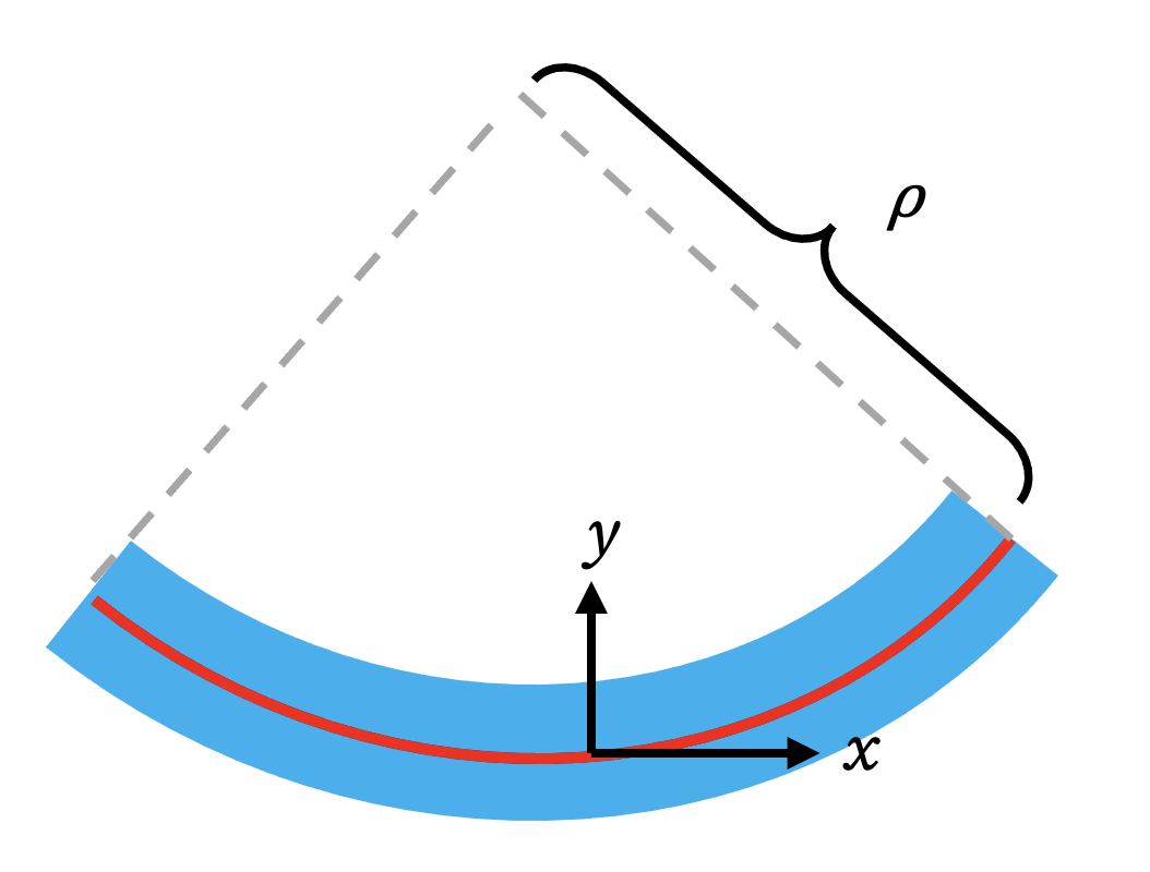
This simple and powerful relationship shows that the strain is zero at the neutral axis (y=0), and it increases linearly as we move away from it.
For mathematical convenience in structural mechanics, it is common to work with a quantity called curvature, denoted by κ (kappa) (see here). Curvature is simply the reciprocal of the radius of curvature: \[ \kappa = \frac{1}{\rho} \] This means that a gentle bend (large ρ) has a small curvature, while a sharp bend (small ρ) has a large curvature. Using this definition, our strain equation becomes: \[ \epsilon_{xx} = -y \kappa \]
The final crucial step is to relate this physical curvature to the beam’s transverse displacement function, v(x). For the small deflections assumed in Euler-Bernoulli theory, there is a direct mathematical approximation: \[ \kappa =\frac{\dfrac{d^2 v}{dx^2}}{\left[1+\left(\dfrac{dv}{dx}\right)^2\right]^{\frac{3}{2}}}\approx \frac{d^2v}{dx^2} \]
Combining these relationships gives us the final, essential equation that links the internal strain to the second derivative of the displacement field. This is the equation that forms the basis of our finite element derivation:
\[ \epsilon_{xx}(x,y) = -y \frac{d^2v}{dx^2} \]
2. Element Definition and Degrees of Freedom (DOFs)
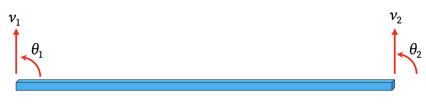
To capture bending behavior, we define a two-node beam element. Each node requires two degrees of freedom (DOFs) to describe its state:
- A transverse displacement,
v. - A rotation,
θ.
For small angles, the rotation is equal to the slope of the displacement curve, so θ = dv/dx.
This means a single beam element has a total of four degrees of freedom. These are collected in the element’s generalized nodal displacement vector, q:
\[ \mathbf{q} = \begin{bmatrix} v_1 \\ \theta_1 \\ v_2 \\ \theta_2 \end{bmatrix} = \begin{bmatrix} v(0) \\ v'(0) \\ v(L) \\ v'(L) \end{bmatrix} \]
3. The Displacement Field and the Need for Hermite Shape Functions
The core of the finite element method is to approximate the continuous displacement field v(x) using a finite number of nodal parameters. A simple linear function is insufficient because its second derivative is always zero, implying zero curvature and thus zero bending strain.
The simplest polynomial that can represent a non-zero, varying curvature is a cubic polynomial, which has four unknown coefficients (a₀ to a₃). This conveniently matches our four nodal DOFs. \[ v(x) = a_0 + a_1 x + a_2 x^2 + a_3 x^3 \]
While we could work with the a_i coefficients, it is far more effective to formulate the problem using shape functions that directly relate the displacement v(x) to the nodal DOFs in the vector q. The specific shape functions used for this are called Hermite Polynomials.
Unlike simpler Lagrange shape functions that only interpolate values, Hermite shape functions interpolate both values and their first derivatives at the nodes. This is exactly what we need to handle both displacement (v) and rotation (θ = dv/dx). The most important consequence is that Hermite polynomials guarantee C¹ continuity between adjacent elements, ensuring that the slope is continuous across nodes and the deformed shape is smooth.
4. Step-by-Step Derivation of the Hermite Shape Functions
We will derive the four shape functions, N₁(x) through N₄(x), such that: \[ \begin{aligned} v(x) &= N_1(x)v_1 + N_2(x)\theta_1 + N_3(x)v_2 + N_4(x)\theta_2\\ &=\langle N_1 \quad N_2 \quad N_3\quad N_4\rangle \begin{Bmatrix} v_1 \\ \theta_1\\ v_2\\ \theta_2 \end{Bmatrix} \end{aligned} \]
Each \(N_i(x)\) is obtained by assuming \(v(x)=a_0+a_1x+a_2x^2+a_3x^3\) and solving for four coefficients such that \(q_i=1\) and all other degrees of freedom (\(q_j=0,\ j\neq i\)) are zero.
Let’s derive N₁(x) by finding a unique cubic polynomial that corresponds to a unit displacement at node 1 (v₁=1) while all other nodal DOFs are zero.
Step 1: Define the Nodal Conditions for N₁(x) The function must satisfy: 1. N₁(0) = 1 (Unit displacement at node 1) 2. N₁'(0) = 0 (Zero slope at node 1) 3. N₁(L) = 0 (Zero displacement at node 2) 4. N₁'(L) = 0 (Zero slope at node 2)
Step 2: Apply Conditions to a General Cubic Polynomial Let N₁(x) = a x³ + b x² + c x + d. Its derivative is N₁'(x) = 3a x² + 2b x + c.
Apply the four conditions: 1. N₁(0) = 1 => a(0) + b(0) + c(0) + d = 1 => d = 1 2. N₁'(0) = 0 => 3a(0) + 2b(0) + c = 0 => c = 0 3. N₁(L) = 0 => aL³ + bL² + 0*L + 1 = 0 => aL³ + bL² = -1 4. N₁'(L) = 0 => 3aL² + 2bL + 0 = 0 => 3aL² + 2bL = 0
Step 3: Solve for the Coefficients a and b From condition (4), we get b = - (3/2)aL. Substitute this into condition (3): aL³ + (-3/2 * aL)L² = -1 aL³ - 3/2 * aL³ = -1 -1/2 * aL³ = -1 => a = 2/L³
Now find b: b = -3/2 * (2/L³) * L => b = -3/L²
Step 4: Assemble the Shape Function N₁(x) Substitute the coefficients a, b, c, d back into the polynomial form:
\[ N_1(x) = \left(\frac{2}{L^3}\right)x^3 - \left(\frac{3}{L^2}\right)x^2 + 1 \]
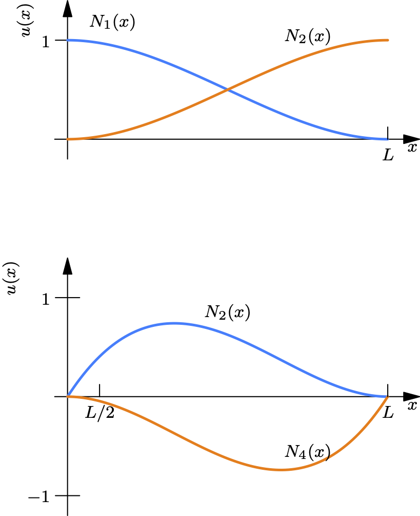
By following the same procedure for the other three unit cases, we derive all four Hermite shape functions.
\[ \boxed{ \begin{aligned} N_1(x) &= 1 - \frac{3x^2}{L^2} + \frac{2x^3}{L^3} \\ N_2(x) &= x - \frac{2x^2}{L} + \frac{x^3}{L^2} \\ N_3(x) &= \frac{3x^2}{L^2} - \frac{2x^3}{L^3} \\ N_4(x) &= -\frac{x^2}{L} + \frac{x^3}{L^2} \end{aligned} } \]
5. Deriving the Element Stiffness Matrix
The final step is to use these shape functions to derive the element stiffness matrix from the fundamental integral: \[ \mathbf{K} = \int_{\Omega} \mathbf{B}^{\mathsf T} \mathbf{E} \mathbf{B} \,dV \]
1. Define the B Matrix: The strain is \(\epsilon_{xx}=-y\dfrac{d^2 v}{dx^2}\) and \(v =\langle N_1 \quad N_2\quad N_3\quad N_4\rangle \mathbf{q}\). The curvature d²v/dx² is: \[ \frac{d^2v}{dx^2} = \frac{d^2}{dx^2}\left(\sum N_i q_i\right) = \begin{bmatrix} N_1'' & N_2'' & N_3'' & N_4'' \end{bmatrix} \mathbf{q} \] The strain-displacement matrix B is therefore: \[ \bbox[5px,border:1px #f2f2f2;background-color:#f2f2f2]{\mathbf{B}(x, y) = -y \begin{bmatrix} \dfrac{d^2N_1}{dx^2} & \dfrac{d^2N_2}{dx^2} & \dfrac{d^2N_3}{dx^2} & \dfrac{d^2N_4}{dx^2} \end{bmatrix}} \]
2. Set up the Stiffness Integral: The volume differential is dV = dA dx. For a 1D stress state, the elasticity matrix E is just Young’s Modulus, E. \[ \mathbf{K} = \int_0^L \int_A (\mathbf{B})^{\mathsf T}_{4\times 1} E \ (\mathbf{B})_{1\times 4} \,dA \,dx \] Substituting the expression for B: \[ \mathbf{K} = \int_0^L \int_A \left( -y \begin{bmatrix} N_1'' \dots \end{bmatrix}^{\mathsf T} \right) E \left( -y \begin{bmatrix} N_1'' \dots \end{bmatrix} \right) \,dA \,dx \] The terms that do not depend on the area (A) can be moved outside the inner integral: \[ \mathbf{K} = \int_0^L \begin{bmatrix} N_1'' \dots \end{bmatrix}^{\mathsf T} E \left( \int_A y^2 \,dA \right) \begin{bmatrix} N_1'' \dots \end{bmatrix} \,dx \]
3. The Final Result: We recognize that the term \(\displaystyle \int_A y^2 dA\) is the definition of the second moment of area, I. This simplifies the integral enormously: \[ \mathbf{K} = \int_0^L \left[ \frac{d^2\mathbf{N}}{dx^2} \right]^{\mathsf T} E I \left[ \frac{d^2\mathbf{N}}{dx^2} \right] \,dx \] Evaluating the second derivatives of the four Hermite shape functions, forming the matrix products, and integrating with respect to x from 0 to L finally yields the classic 4x4 Euler-Bernoulli beam stiffness matrix:
\[ \bbox[5px,border:1px #f2f2f2;background-color:#f2f2f2]{ \mathbf{K} = \frac{EI}{L^3} \begin{bmatrix} 12 & 6L & -12 & 6L \\ 6L & 4L^2 & -6L & 2L^2 \\ -12 & -6L & 12 & -6L \\ 6L & 2L^2 & -6L & 4L^2 \end{bmatrix} } \] * Sometimes, we put a subscript e (as \(\mathbf{K}_e\)) to indicate that the above matrix is the stiffness matrix of an element.
Arbitrary Oriented Beam and Transformation Matrix
If we consider 6 degrees of freedom (considering beam-column element), which the beam can be stretched or compressed as well, then the stiffness matrix of the element is \[ \mathbf{K}_e^{\text{local}} = \begin{bmatrix} \dfrac{EA}{L} & 0 & 0 & -\dfrac{EA}{L} & 0 & 0 \\[1em] 0 & \dfrac{12EI}{L^3} & \dfrac{6EI}{L^2} & 0 & -\dfrac{12EI}{L^3} & \dfrac{6EI}{L^2} \\[1em] 0 & \dfrac{6EI}{L^2} & \dfrac{4EI}{L} & 0 & -\dfrac{6EI}{L^2} & \dfrac{2EI}{L} \\[1em] -\dfrac{EA}{L} & 0 & 0 & \dfrac{EA}{L} & 0 & 0 \\[1em] 0 & -\dfrac{12EI}{L^3} & -\dfrac{6EI}{L^2} & 0 & \dfrac{12EI}{L^3} & -\dfrac{6EI}{L^2} \\[1em] 0 & \dfrac{6EI}{L^2} & \dfrac{2EI}{L} & 0 & -\dfrac{6EI}{L^2} & \dfrac{4EI}{L} \end{bmatrix} \]
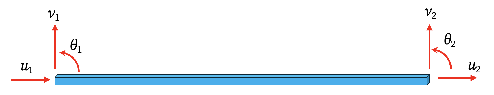
Now let’s consider a beam which makes an angle \(\alpha\) with the global \(x\)-axis. In this case, we have to rotate the global coordinate system (x, y) by an angle \(\alpha\) to reach the local system (x', y').
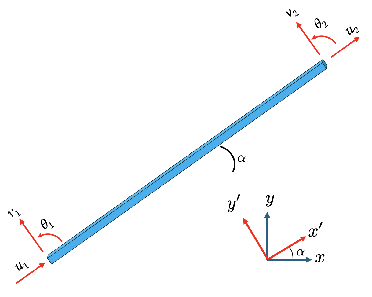
The transformation of the degrees of freedom \(u\) and \(v\) is the same as the transformation of u and v for a truss element. Since the degree of freedom \(\theta\) is the same in both coordinate system, the transformation matrix becomes
\[ \mathbf{T}=\begin{bmatrix} c & s & 0 & 0 & 0 & 0\\ -s & c & 0 & 0 & 0 & 0\\ 0 & 0 & 1 & 0 & 0 & 0\\ 0 & 0 & 0& c & s & 0 \\ 0 & 0 & 0 & -s & c & 0 \\ 0 & 0& 0 & 0 & 0 & 1 \end{bmatrix} \] where \[ c=\cos\alpha,\qquad s=\sin\alpha. \] The stiffness matrix in the global coordinate system becomes \[ \mathbf{K}_e^{\text{global}}=\mathbf{T}^{\mathsf T} \mathbf{K}_e^{\text{local}} \mathbf{T} \]