In this section we introduce a notion that is basic to the theory of random processes, the notion of the conditional probability of a random event \(A\) , given a random variable \(X\) . This notion forms the basis of the mathematical treatment of jointly distributed random variables that are not independent and, consequently, are dependent.
Given two events, \(A\) and \(B\) , on the same probability space, the conditional probability \(P[A \mid B]\) of the event \(A\) , given the event \(B\) , has been defined: \[P[A \mid B]=\left\{\begin{aligned} &\frac{P[A B]}{P[B]} &&\text {if } P[B]>0 \\ &\text {undefined} &&\text{if } P[B]=0. \end{aligned}\right. \tag{11.1}\]
Now suppose we are given an event \(A\) and a random variable \(X\) , both defined on the same probability space. We wish to define, for any real number \(x\) , the conditional probability of the event \(A\) , given the event that the observed value of \(X\) is equal to \(x\) , denoted in symbols by \(P[A \mid X=x]\) . Now if \(P[X=x]>0\) , we may define this conditional probability by (11.1). However, for any random variable \(X, P[X=x]=0\) for all (except, at most, a countable number of) values of \(x\) . Consequently, the conditional probability \(P[A \mid X=x]\) of the event \(A\) , given that \(X=x\) , must be regarded as being undefined insofar as (11.1) is concerned.
The meaning that one intuitively assigns to \(P[A \mid X=x]\) is that it represents the probability that \(A\) has occurred, knowing that \(X\) was observed as equal to \(x\) . Therefore, it seems natural to define
\[P[A \mid X=x]=\lim _{h \rightarrow 0} P[A \mid x-h
if the conditioning events \([x-h
Given a real number \(x\) , define \(H_{n}(x)\) as that interval, of length \(1 / 2^{n}\) , starting at a multiple of \(1 / 2^{n}\) , that contains \(x\) ; in symbols,
\[H_{n}(x)=\left\{x^{\prime}: \frac{\left[x \cdot 2^{n}\right]}{2^{n}} \leq x^{\prime}<\frac{\left[x \cdot 2^{n}\right]+1}{2^{n}}\right\}. \tag{11.3}\]
Then we define the conditional probability of the event \(A\) , given that the random variable \(X\) has an observed value equal to \(x\) , by
\[P[A \mid X=x]=\lim _{n \rightarrow \infty} P\left[A \mid X \text { is in } H_{n}(x)\right]. \tag{11.4}\]
It may be proved that the conditional probability \(P[A \mid X=x]\) , defined by (11.4), has the following properties.
First, the convergence set \(C\) of points \(x\) on the real line at which the limit in (11.4) exists has probability one, according to the probability function of the random variable \(X\) ; that is, \(P_{X}[C]=1\) . For practical purposes this suffices, since we expect that all observed values of \(X\) lie in the set \(C\) , and we wish to define \(P[A \mid X=x]\) only at points \(x\) that could actually arise as observed values of \(X\) .
Second, from a knowledge of \(P[A \mid X=x]\) one may obtain \(P[A]\) by the following formulas:
\[P[A]=\left\{\begin{aligned} &\int_{-\infty}^{\infty} P[A \mid X=x] d F_{X^{\prime}}(x) \\[5mm] &\int_{-\infty}^{\infty} P[A \mid X=x] f_{X^{\prime}}(x) d x \\[5mm] &\sum_{\substack{\text { over all } x \text { such } \\ \text { that } p_{X}(x)>0}} P[A \mid X=x] p_{X}(x) \end{aligned}\right.\tag{11.5}\]
in which the last two equations hold if \(X\) is respectively continuous or discrete. More generally, for every Borel set \(B\) of real numbers, the probability of the intersection of the event \(A\) and the event \(\{X\) is in \(B\}\) that the observed value of \(X\) is in \(B\) is given by
\[P[A\{X \text { is in } B\}]=\int_{B} P[A \mid X=x] d F_{X}(x). \tag{11.6}\]
Indeed, in advanced studies of probability theory the conditional probability \(P[A \mid X=x]\) is defined not constructively by (11.4) but descriptively, as the unique (almost everywhere) function of \(x\) satisfying (11.6) for every Borel set \(B\) of real numbers. This characterization of \(P[A \mid X=x]\) is used to prove (11.15).
Example 11A . A young man and a young lady plan to meet between 5:00 and 6:00 P.M., each agreeing not to wait more than ten minutes for the other. Assume that they arrive independently at random times between 5:00 and 6:00 P.M. Find the conditional probability that the young man and the young lady will meet, given that the young man arrives at 5:30 P.M.
Solution
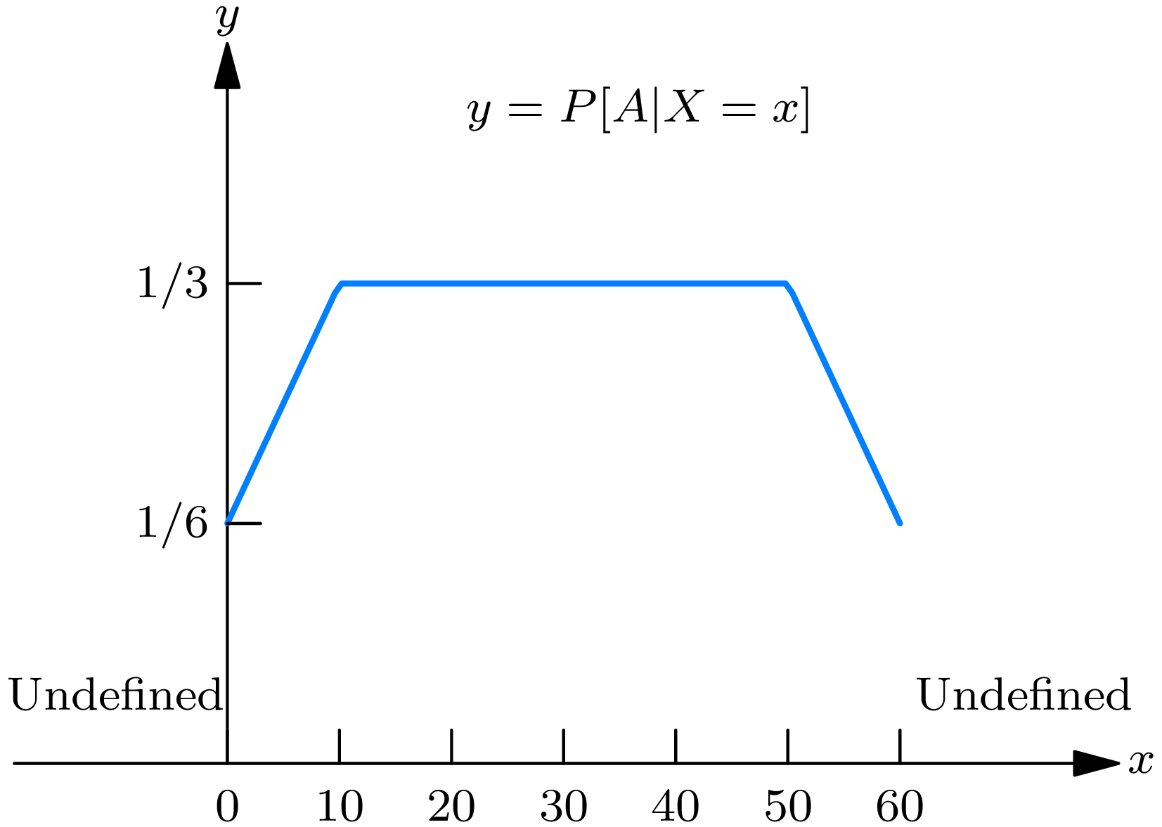
Let \(X\) be the man’s arrival time (in minutes after 5:00 p.M.) and let \(Y\) be the lady’s arrival time (in minutes after 5:00 P.M.). If the man arrives at a time \(x\) , there will be a meeting if and only if the lady’s arrival time \(Y\) satisfies \(|Y-x| \leq 10\) or \(-10+x \leq Y \leq x+10\) . Let \(A\) denote the event that the man and lady meet. Then, for any \(x\) between 0 and 60 \begin{align} P[A \mid X=x] & =P[-10 \leq Y-X \leq 10 \mid X=x] \tag{11.7}\\ & =P[-10+x \leq Y \leq x+10 \mid X=x] \\ & =P[-10+x \leq Y \leq x+10], \end{align} in which we have used (11.9) and (11.11). Next, using the fact that \(Y\) is uniformly distributed between 0 and 60, we obtain (as graphed in Fig. 11A) \[P[A \mid X = x] \left\{ \begin{aligned} &\frac{10 + x}{60}, && \text{if } 0 \leq x \leq 10 \\ &\frac{1}{3}, && \text{if } 10 \leq x \leq 50 \\ &\frac{70 - x}{60}, && \text{if } 50 \leq x \leq 60 \\ &\text{undefined}, && \text{if } x < 0 \text{ or } x > 60, \end{aligned}\right. \tag{11.8}\] Consequently, \(P[A \mid X=30]=\frac{1}{3}\) , so that the conditional probability that the young man and the young lady will meet, given that the young man arrives at 5:30 P.M., is \(\frac{1}{3}\) . Further, by applying (11.5), we determine that \(P[A]=\frac{11}{36}\) .
In (11.7) we performed certain manipulations that arise frequently when one is dealing with conditional probabilities. We now justify these manipulations.
Consider two jointly distributed random variables \(X\) and \(Y\) . Let \(g(x, y)\) be a Borel function of two variables. Let \(z\) be a fixed real number. Let \(A=[g(X, Y) \leq z]\) be the event that the random variable \(g(X, Y)\) has an observed value less than or equal to \(z\) . Next, let \(x\) be a fixed real number, and let \(A(x)=[g(x, Y) \leq z]\) be the event that the random variable \(g(x, Y)\) , which is a function only of \(Y\) , has an observed value less than or equal to \(z\) . It appears formally reasonable that
\[P[g(X, Y) \leq z \mid X=x]=P[g(x, Y) \leq z \mid X=x] . \tag{11.9}\]
In words, a statement involving the random variable \(X\) , conditioned by the hypothesis that the value of \(X\) is a given number \(x\) , has the same conditional probability given \(X=x\) , as the corresponding statement obtained by replacing the random variable \(X\) by its observed value. The proof of (11.9) is omitted, since it is beyond the scope of this book.
It may help to comprehend (11.9) if we state it in terms of the events \(A=[g(X, Y) \leq z]\) and \(A(x)=[g(x, Y) \leq z]\) . Equation (11.9) asserts that the functions of \(u\) ,
\[P[A \mid X=u] \quad \text { and } \quad P[A(x) \mid X=u] \tag{11.10}\]
have the same value at \(u=x\) .
Another important formula is the following. If the random variables \(X\) and \(Y\) are independent, then
\[P[g(x, Y) \leq z \mid X=x]=P[g(x, Y) \leq z], \tag{11.11}\]
since it holds that
\[P[A \mid X=x]=P[A] \quad \text{if the event} \;A ; \text{is independent of}; X, \tag{11.12}\]
We thus obtain the basic fact that if the random variables \(X\) and \(Y\) are independent \[P[g(X, Y) \leq z|X=x] = P[g(x, Y) \leq z | X=x]=P[g(x, Y) \leq z]. \tag{11.13}\]
We next define the notion of the the conditional distribution function of one random variable \(Y\) given another random variable \(X\) , denoted \(F_{Y \mid X}(.|.)\) For any real numbers \(x\) and \(y\) , it is defined by
\[F_{Y \mid X}(y \mid x)=P[Y \leq y \mid X=x]. \tag{11.14}\]
The conditional distribution function \(F_{Y \mid X}(.|.)\) has the basic property that for any real numbers \(x\) and \(y\) the joint distribution function \(F_{X, Y}(x, y)\) may be expressed in terms of \(F_{Y \mid X}(y \mid x)\) by
\[F_{X, Y}(x, y)=\int_{-\infty}^{x} F_{Y \mid X}\left(y \mid x^{\prime}\right) d F_{X}\left(x^{\prime}\right). \tag{11.15}\]
To prove (11.15), let \(X\) and \(Y\) be two jointly distributed random variables. For two given real numbers \(x\) and \(y\) define \(A=[Y \leq y]\) . Then (11.15) may be written
\[P[X \leq x, Y \leq y]=\int_{-\infty}^{x} P\left[A \mid X=x^{\prime}\right] d F_{X}\left(x^{\prime}\right). \tag{11.16}\]
If in (11.6) \(B=\left\{x^{\prime}: \ x^{\prime} \leq x\right\},\) (11.16) is obtained.
Now suppose that the random variables \(X\) and \(Y\) are jointly continuous. We may then define the conditional probability density function of the random variable \(Y\) , given the random variable \(X\) , denoted by \(f_{Y \mid X}(y \mid x)\) . It is defined for any real numbers \(x\) and \(y\) by
\[f_{Y\mid X}(y \mid x)=\frac{\partial}{\partial y} F_{Y \mid X}(y \mid x). \tag{11.17}\]
We now prove the basic formula: if \(f_{X}(x)>0\) , then
\[f_{Y \mid X}(y \mid x)=\frac{f_{X, Y}(x, y)}{f_{X}(x)}. \tag{11.18}\]
To prove (11.18), we differentiate (11.15) with respect to \(x\) (first replacing \(d F_{X}\left(x^{\prime}\right)\) by \(\left.f_{X}\left(x^{\prime}\right) d x^{\prime}\right)\) ). Then
\[\frac{\partial}{\partial x} F_{X, Y}(x, y)=F_{Y \mid X}(y \mid x) f_{X}(x) \tag{11.19}\]
Now differentiating (11.19) with respect to \(y\) , we obtain
\[f_{X, Y}(x, y)=f_{Y \mid X}(y \mid x) f_{X}(x) \tag{11.20}\]
from which (11.18) follows immediately.
Example 11B . Let \(X_{1}\) and \(X_{2}\) be jointly normally distributed random variables whose probability density function is given by (9.31). Then the conditional probability density of \(X_{1}\) , given \(X_{2}\) , is equal to
\begin{align} & f_{X_{1} \mid X_{2}}(x \mid y)=\frac{1}{\sqrt{2 \pi} \sigma_{1} \sqrt{1-\rho^{2}}} \tag{11.21}\\[3mm] & \quad \times \exp \left\{-\frac{1}{2\left(1-\rho^{2}\right) \sigma_{1}^{2}}\left[x-m_{1}-\rho \frac{\sigma_{1}}{\sigma_{2}}\left(y-m_{2}\right)\right]^{2}\right\} \end{align}
In words, the conditional probability law of the random variable \(X_{1}\) , given \(X_{2}\) , is the normal probability law with parameters \(m=m_{1}+\rho\left(\sigma_{1} / \sigma_{2}\right)\) \(\left(x_{2}-m_{2}\right)\) and \(\sigma=\sigma_{1} \sqrt{1-\rho^{2}}\) . To prove (11.21), one need only verify that it is equal to the quotient \(f_{X_{1}, X_{2}}(x, y) \mid f_{X_{2}}(y)\) . Similarly, one may establish the following result.
Example 11C . Let \(X\) and \(Y\) be jointly distributed random variables. Let
\[R=\sqrt{X^{2}+Y^{2}}, \quad \theta=\tan ^{-1}(Y / X). \tag{11.22}\]
Then, for \(r>0\)
\[f_{\theta \mid R}(\theta \mid r)=\frac{f_{X, Y}(r \cos \theta, r \sin \theta)}{\displaystyle \int_{0}^{2 \pi} d \theta f_{X, Y}(r \cos \theta, r \sin \theta)}. \tag{11.23}\]
In the foregoing examples we have considered the problem of obtaining \(f_{X \mid Y}(x \mid y)\) , knowing \(f_{X, Y}(x, y)\) . We next consider the converse problem of obtaining the individual probability law of \(X\) from a knowledge of the conditional probability law of \(X\) , given \(Y\) , and of the individual probability law of \(Y\) .
Example 11D . Consider the decay of particles in a cloud chamber (or, similarly the breakdown of equipment or the occurrence of accidents). Assume that the time \(X\) of any particular particle to decay is a random variable obeying an exponential probability law with parameter \(y\) . However, it is not assumed that the value of \(y\) is the same for all particles. Rather, it is assumed that there are particles of different types (or equipment of different types or individuals of different accident proneness). More specifically, it is assumed that for a particle randomly selected from the cloud chamber the parameter \(y\) is a particular value of a random variable \(Y\) obeying a gamma probability law with a probability density function,
\[f_{Y}(y)=\frac{\beta^{\alpha}}{\Gamma(\alpha)} y^{\alpha-1} e^{-\beta y}, \quad \text { for } y>0, \tag{11.24}\]
in which the parameters \(\alpha\) and \(\beta\) are positive constants characterizing the experimental conditions under which the particles are observed.
The assumption that the time \(X\) of a particle to decay obeys an exponential law is now expressed as an assumption on the conditional probability law of \(X\) given \(Y\) :
\[f_{X \mid Y}(x \mid y)=y e^{-x y} \quad \text { for } x>0. \tag{11.25}\]
We find the individual probability law of the time \(X\) (of a particle selected at random to decay) as follows; for \(x>0\)
\begin{align} f_{X}(x) & =\int_{-\infty}^{\infty} f_{X, Y}(x, y) d y=\int_{-\infty}^{\infty} f_{X \mid Y}(x \mid y) f_{Y}(y) d y \tag{11.26}\\[3mm] & =\int_{0}^{\infty} y e^{-x y} \frac{\beta^{\alpha}}{\Gamma(\alpha)} y^{\alpha-1} e^{-\beta y} d y \\[3mm] & =\frac{\alpha \beta^{\alpha}}{(\beta+x)^{\alpha+1}}. \end{align}
The reader interested in further study of the foregoing model, as well as a number of other interesting topics, should consult J. Neyman, “The Problem of Inductive Inference”, Communications on Pure and Applied Mathematics , Vol. 8 (1955), pp. 13–46.
The foregoing notions may be extended to several random variables. In particular, let us consider \(n\) random variables \(X_{1}, X_{2}, \ldots, X_{n}\) and a random variable \(U\) , all of which are jointly distributed. By suitably adapting the foregoing considerations, we may define a function
\[F_{X_{1}, X_{2}, \ldots, X_{n} \mid U}\left(x_{1}, x_{2}, \ldots, x_{n} \mid u\right), \tag{11.27}\]
called the conditional distribution function of the random variables \(X_{1}, X_{2}, \ldots, X_{n}\) , given the random variable \(U\) , which may be shown to satisfy, for all real numbers \(x_{1}, x_{2}, \ldots, x_{n}\) and \(u\) ,
\begin{align} F_{X_{1}, \ldots, X_{n}, U}\left(x_{1}, \ldots,\right. & \left.x_{n}, u\right) \tag{11.28}\\ & =\int_{-\infty}^{u} F_{X_{1}, \ldots, X_{n} \mid U}\left(x_{1}, \ldots, x_{n} \mid u^{\prime}\right) d F_{U}\left(u^{\prime}\right). \end{align}
Theoretical Exercises
11.1 . Let \(T\) be a random variable, and let \(t\) be a fixed number. Define the random variable \(U\) by \(U=T-t\) and the event \(A\) by \(A=[T>t]\) . Evaluate \(P[A \mid U=x]\) and \(P[U>x \mid A]\) in terms of the distribution function of \(T\) . Explain the difference in meaning between these concepts.
11.2 . If \(X\) and \(Y\) are independent Poisson random variables, show that the conditional distribution of \(X\) , given \(X+Y\) , is binomial.
11.3 . Given jointly distributed random variables, \(X_{1}\) and \(X_{2}\) , prove that, for any \(x_{2}\) and almost all \(x_{1}, F_{X_{2} \mid X_{1}}\left(x_{2} \mid x_{1}\right)=F_{X_{2}}\left(x_{2}\right)\) if and only if \(X_{1}\) and \(X_{2}\) are independent.
11.4 . Prove that for any jointly distributed random variables \(X_{1}\) and \(X_{2}\)
\[\int_{-\infty}^{\infty} f_{X_{1} \mid X_{2}}\left(x_{1} \mid x_{2}\right) d x_{1}=1, \quad \int_{-\infty}^{\infty} f_{X_{2} \mid X_{1}}\left(x_{2} \mid x_{1}\right) d x_{2}=1.\]
For contrast evaluate
\[\int_{-\infty}^{\infty} f_{X_{1} \mid X_{2}}\left(x_{1} \mid x_{2}\right) d x_{2}, \quad \int_{-\infty}^{\infty} f_{X_{2} \mid X_{1}}\left(x_{2} \mid x_{1}\right) d x_{1}.\]
Exercises
In exercises 11.1 to 11.3 let \(X\) and \(Y\) be independent random variables. Let \(Z=Y-X\) . Let \(A=[|Y-X| \leq 1]\) . Find (i) \(P[A \mid X=1]\) , (ii) \(F_{Z \mid X}(0 \mid 1)\) , (iii) \(f_{Z \mid X}(0 \mid 1)\) , (iv) \(P[Z \leq 0 \mid A]\) .
11.1 . If \(X\) and \(Y\) are each uniformly distributed over the interval 0 to 2.
Answer
(i) 1; (ii), (iii), (iv) \(\frac{1}{2}\) .
11.2 . If \(X\) and \(Y\) are each normally distributed with parameters \(m=0\) and \(\sigma=2\) .
11.3 . If \(X\) and \(Y\) are each exponentially distributed with parameter \(\dot{\lambda}=1\) .
Answer
(i) 0.865; (ii) 0.632; (iii) 0.368; (iv) 0.5.
In exercises 11.4 to 11.6 let \(X\) and \(Y\) be independent random variables. Let \(U=X+Y\) and \(V=Y-X\) . Let \(A=[|V| \leq 1]\) . Find (i) \(P[A \mid U=1]\) , (ii) \(F_{\mathrm{I}^{\prime} \mid l}(0 \mid 1)\) , (iii) \(f_{\mathrm{I}^{-} \mid l}(0 \mid 1)\) , (iv) \(P[U \geq 0 \mid A]\) , (v) \(f_{\mathrm{V} \mid U}(v \mid u)\) .
11.4 . If \(X\) and \(Y\) are each uniformly distributed over the interval 0 to 2.
11.5 . If \(X\) and \(Y\) are each normally distributed with parameters \(m=0\) and \(\sigma=2\) .
Answer
(i) 0.276; (ii) 0.5; (iii) 0.2; (iv) 0.5, (v) \(\frac{1}{2} \phi(v / 2)\) .
11.6 . If \(X\) and \(Y\) are each exponentially distributed with parameter \(\lambda=1\) .
11.7 . Let \(X_{1}\) and \(X_{2}\) be jointly normally distributed random variables (representing the observed amplitudes of a noise voltage recorded a known time interval apart). Assume that their joint probability density function is given by (9.31) with (i) \(m_{1}=m_{2}=0, \sigma_{1}=\sigma_{2}=1, \rho=0.5\) , (ii) \(m_{1}=1\) , \(m_{2}=2, \sigma_{1}=1, \sigma_{2}=4, \rho=0.5\) . Find \(P\left[X_{2}>1 \mid X_{1}=1\right]\) .
Answer
(i) 0.28; (ii) 0.61.
11.8 . Let \(X_{1}\) and \(X_{2}\) be jointly normally distributed random variables, representing the daily sales (in thousands of units) of a certain product in a certain store on two successive days. Assume that the joint probability density function of \(X_{1}\) and \(X_{2}\) is given by (9.31), with \(m_{1}=m_{2}=3, \sigma_{1}=\sigma_{2}=1\) , \(\rho=0.8\) . Find \(K\) so that (i) \(P\left[X_{2}>K\right]=0.05\) , (ii) \(P\left[X_{2}>K \mid X_{1}=2\right]=\) 0.05, (iii) \(P\left[X_{2} \geq K \mid X_{1}=1\right]=0.05\) . Suppose the store desires to have on hand on a given day enough units of the product so that with probability 0.95 it can supply all demands for the product on the day. How large should its inventory be on a given morning if (iv) yesterday’s sales were 2000 units, (v) yesterday’s sales are not known.