Some understanding of the kinds of random phenomena that obey the normal probability law can be obtained by examining the manner in which the normal density function and the normal distribution function first arose in probability theory as means of approximately evaluating probabilities associated with the binomial probability law.
The following theorem was stated by de Moivre in 1733 for the case \(p=\frac{1}{2}\) and proved for arbitrary values of \(p\) by Laplace in 1812.
The probability that a random phenomenon obeying the binomial probability law with parameters \(n\) and \(p\) will have an observed value lying between a and \(b\) , inclusive, for any two integers \(a\) and \(b\) , is given approximately by \begin{align} \sum_{k=a}^{b}\left(\begin{array}{l} n \\ k \end{array}\right) p^{k} q^{n-k} & \doteq \frac{1}{\sqrt{2 \pi}} \int_{\frac{a-n p-1 / 2}{\sqrt{n p q}}}^{\frac{b-n p+1 / 2}{\sqrt{n p q}}} e^{-1 / 2 y^{2}} d y \tag{2.1} \\ & =\Phi\left(\frac{b-n p+\frac{1}{2}}{\sqrt{n p q}}\right)-\Phi\left(\frac{a-n p-\frac{1}{2}}{\sqrt{n p q}}\right) \end{align}
Before indicating the proof of this theorem, let us explain its meaning and usefulness by the following examples.
Example 2A. Suppose that \(n=6000\) tosses of a fair die are made. The probability that exactly \(k\) of the tosses will result in a “three” is given by \(\left(\begin{array}{c}6000 \\ k\end{array}\right)\left(\frac{1}{6}\right)^{k}\left(\frac{5}{6}\right)^{6000-k}\) The probability that the number of tosses on which a “three” will occur is between 980 and 1030, inclusive, is given by the sum
\[\sum_{k=980}^{1030}\left(\begin{array}{c} 6000 \tag{2.2} \\ k \end{array}\right)\left(\frac{1}{6}\right)^{k}\left(\frac{5}{6}\right)^{6000-k}\]
It is clearly quite laborious to evaluate this sum directly. Fortunately, by (2.1), the sum in (2.2) is approximately equal to \[\frac{1}{\sqrt{2 \pi}} \int_{\frac{980-1000-1 / 2}{28.87}}^{\frac{1030-1000+1 / 2}{28.87}} e^{- y^{2}/2} d y=\Phi(1.06)-\Phi(-0.71)=0.617.\]
Example 2B. In 40,000 independent tosses of a coin heads appeared 20,400 times. Find the probability that if the coin were fair one would observe in 40,000 independent tosses (i) 20,400 or more heads, (ii) between 19,600 and 20,400 heads.
Solution
Let \(X\) be the number of heads in 40,000 independent tosses of a fair coin. Then \(X\) obeys a binomial probability law with mean \(m=n p=20,000\) , variance \(\sigma^{2}=n p q=10,000\) , and standard deviation \(\sigma=100\) . According to the normal approximation to the binomial probability law, \(X\) approximately obeys a normal probability law with parameters \(m=20,000\) and \(\sigma=100\) [in making this statement we are ignoring the terms in (2.1) involving \(\frac{1}{2}\) , which are known as a “continuity” correction]. Since 20,400 is four standard deviations more then the mean of the probability law of \(X\) , the probability is approximately 0 that one would observe a value of \(X\) more than 20,400. Similarly, the probability is \(1\) that one would observe a value of \(X\) between 19,600 and 20,400.
In order to have a convenient language in which to discuss the proof of (2.1), let us suppose that we are observing the number \(X\) of successes in \(n\) independent repeated Bernoulli trials with probability \(p\) of success at each trial. Next, to each outcome \(X\) let us compute the quantity
\[h=\frac{X-n p}{\sqrt{n p q}}, \tag{2.3}\]
which represents the deviation of \(X\) from \(n p\) divided by \(\sqrt{n p q}\) . Recall that the quantities \(n p\) and \(\sqrt{n p q}\) are equal, respectively, to the mean and standard deviation of the binomial probability law. The deviation \(h\) , defined by (2.3), is a random quantity obeying a discrete probability law specified by a probability mass function \(p^{*}(h)\) , which may be given in terms of the probability mass function \(p(x)\) by
\[p^{*}(h)=p(h \sqrt{n p q}+n p). \tag{2.4}\]
In words, (2.4) expresses the fact that for any given real number \(h\) the probability that the deviation (of the number of successes from \(n p\) , divided by \(\sqrt{n p q}\) ) will be equal to \(h\) is the same as the probability that the number of successes will be equal to \(h \sqrt{n p q}+n p\) .
The advantage in considering the probability mass function \(p^{*}(h)\) over the original probability mass function \(p(x)\) can be seen by comparing their graphs, which are given in Figs. 7.2.1 and 7.2.2 for \(n=50\) and 100 and \(p=\frac{1}{3}\) . The graph of the function \(p(x)\) becomes flatter and flatter and spreads out more and more widely along the \(x\) -axis as the number \(n\) of trials increases.
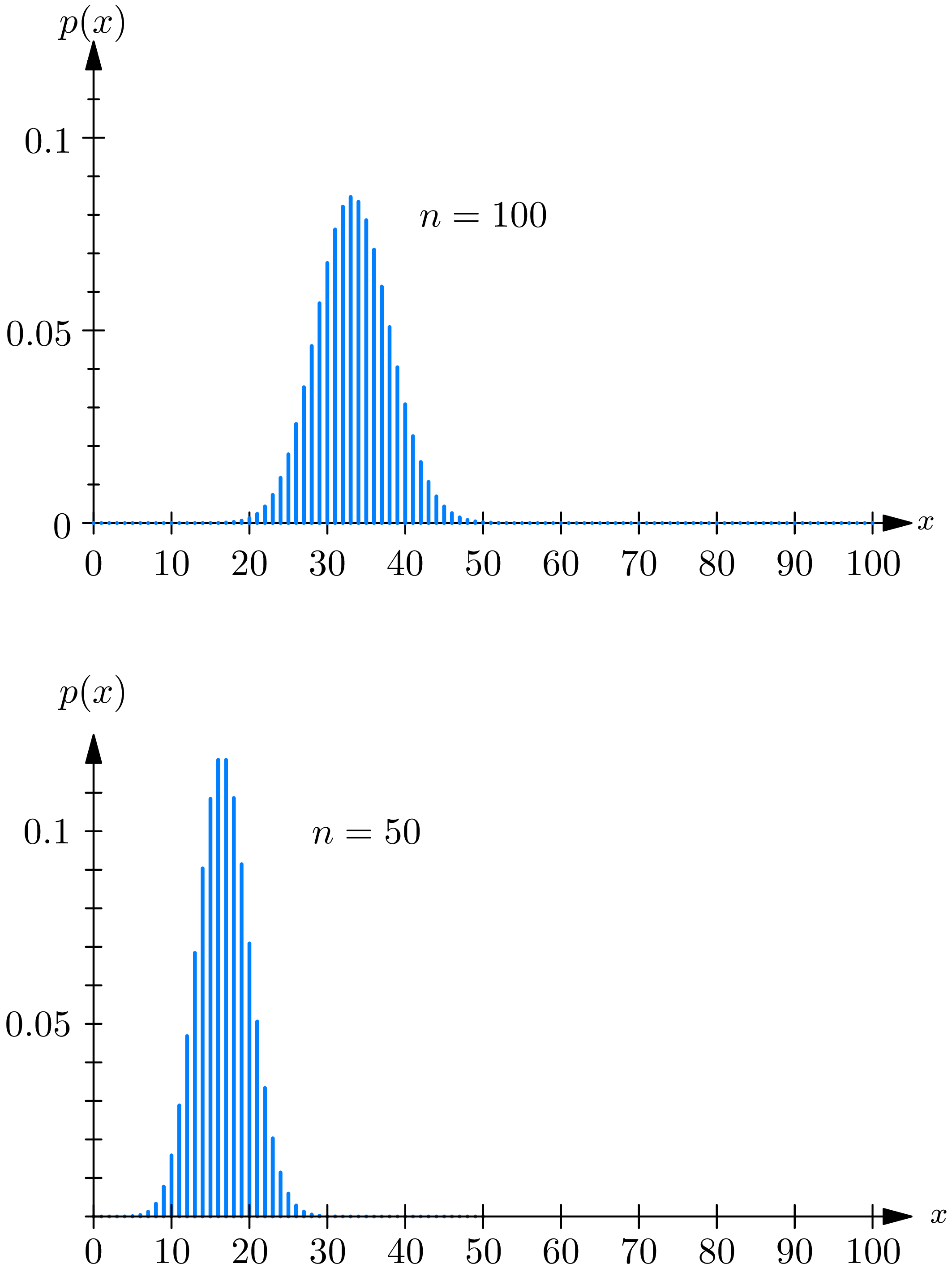

The graphs of the functions \(p^{*}(h)\) , on the other hand, are very similar to each other, for different values of \(n\) , and seem to approach a limit as \(n\) becomes infinite. It might be thought that it is possible to find a smooth curve that would be a good approximation to \(p^{*}(h)\) , at least when the number of trials \(n\) is large. We now show that this is indeed possible. More precisely, we show that if \(h\) is a real number for which \(p^{*}(h)>0\) then, approximately, \[p^{*}(h) \doteq \frac{1}{\sqrt{n p q}} \frac{1}{\sqrt{2 \pi}} e^{-h^{2}/2}, \tag{2.5}\] in the sense that \[\lim _{n \rightarrow \infty} \frac{\sqrt{2 \pi n p q}\ p(h \sqrt{n p q}+n p)}{e^{-1 / 2 h^{2}}}=1. \tag{2.6}\]
To prove (2.6), we first obtain the approximate expression for \(p(x)\) ; for \(k=0,1, \ldots, n\) \[p(k)=\frac{1}{\sqrt{2 \pi}} \sqrt{\frac{n}{k(n-k)}}\left(\frac{n p}{k}\right)^{k}\left(\frac{n q}{n-k}\right)^{n-k} e^{R}, \tag{2.7}\] in which \(|R|<\frac{1}{12}\left(\dfrac{1}{n}+\dfrac{1}{k}+\dfrac{1}{n-k}\right)\) . Equation (2.7) is an immediate consequence of the approximate expression for the binomial coefficient \(\left(\begin{array}{l}n \\ k\end{array}\right)\) ; for any integers \(n\) and \(k=0,1, \ldots, n\) \[\left(\begin{array}{l} n \tag{2.8} \\ k \end{array}\right)=\frac{n !}{k !(n-k) !}=\frac{1}{\sqrt{2 \pi}} \sqrt{\frac{n}{k(n-k)}}\left(\frac{n}{k}\right)^{k}\left(\frac{n}{n-k}\right)^{n-k} e^{R}\]
Equation (2.8), in turn, is an immediate consequence of the approximate expression for \(m\) ! given by Stirling’s formula; for any integer \(m=1,2, \ldots\) . \[m !=\sqrt{2 \pi m} m^{m} e^{-m} e^{r(m)}, \quad 0
If we ignore all terms that tend to 0 as \(n\) tends to infinity in (2.11), we obtain the desired conclusion, namely (2.6) .
From (2.6) one may obtain a proof of (2.1) . However, in this book we give only a heuristic geometric proof that (2.6) implies (2.1) . For an elementary rigorous proof of (2.1) the reader should consult J. Neyman, First Course in Probability and Statistics , New York, Henry Holt, 1950, pp. 234–242. In Chapter 10 we give a rigorous proof of (2.1) by using the method of characteristic functions.
A geometric derivation of (2.1) from (2.6) is as follows. First plot \(p^{*}(h)\) in Fig. 2B as a function of \(h\) ; note that \(p^{*}(h)=0\) for all points \(h\) , except those that may be represented in the form \[h=(k-n p) / \sqrt{n p q} \tag{2.12}\] for some integer \(k=0,1, \ldots, n\) . Next, as in Fig. 2C, plot \(p^{*}(h)\) by a series of rectangles of height \((1 / \sqrt{2 \pi}) e^{-h^{2}/2}\) , centered at all points \(h\) of the form of (2.12).
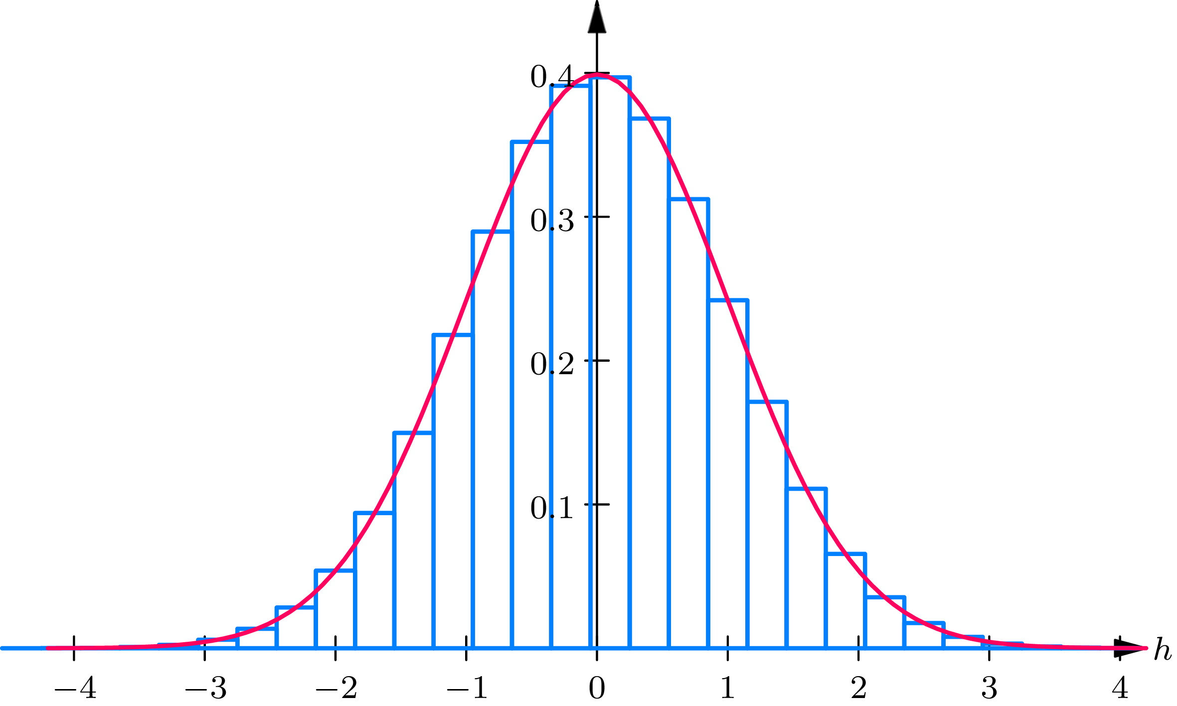
From Fig. 2C we obtain (2.1). It is clear that \[\sum_{k=a}^{b} p(k)=\sum_{\substack{\text { over } h \text { of the form of } \\ \text { (2.12) for } k=a, \ldots, b}} p^{*}(h)\] which is equal to the sum of the areas of the rectangles in Fig.2C centered at the points \(h\) of the form of (2.12), corresponding to the integers \(k\) from \(a\) to \(b\) , inclusive. Now, the sum of the area of these rectangles is an approximating sum to the integral of the function \((1 / \sqrt{2 \pi}) e^{-1 / h^{2}}\) between the limits \(\left(a-n p-\frac{1}{2}\right) / \sqrt{n p q}\) and \(\left(b-n p+\frac{1}{2}\right) / \sqrt{n p q}\) . We have thus obtained the approximate formula (2.1).
It should be noted that we have available two approximations to the probability mass function \(p(x)\) of the binomial probability law. From (2.5) and (2.6) it follows that
\[\left(\begin{array}{l} n \tag{2.13} \\ x \end{array}\right) p^{x} q^{n-x} \doteq \frac{1}{\sqrt{2 \pi n p q}} \exp \left(-\frac{1}{2} \frac{(x-n p)^{2}}{n p q}\right),\]
whereas from (2.1) one obtains, setting \(a=b=x\) ,
\[\left(\begin{array}{l} n \\ x \tag{2.14} \end{array}\right) p^{x} q^{n-x} \doteq \frac{1}{\sqrt{2 \pi}} \int_{\frac{x-n p-1 / 2}{\sqrt{n p q}}}^{\frac{x-n p+1 / 2}{\sqrt{n p q}}} e^{-1 / 2 y^{2}} d y\]
In using any approximation formula, such as that given by (2.1), it is important to have available “remainder terms” for the determination of the accuracy of the approximation formula. Analytic expressions for the remainder terms involved in the use of (2.1) are to be found in J. V. Uspensky, Introduction to Mathematical Probability , McGraw-Hill, New York, 1937, p. 129, and W. Feller, “On the normal approximation to the binomial distribution”, Annals of Mathematical Statistics , Vol. 16, (1945), pp. 319–329. However, these expressions do not lead to conclusions that are easy to state. A booklet entitled Binomial, Normal, and Poisson Probabilities , by Ed. Sinclair Smith (published by the author in 1953 at Bel Air, Maryland), gives extensive advice on how to compute expeditiously binomial probabilities with 3-decimal accuracy. Smith (p. 38) states that (2.1) gives 2-decimal accuracy or better if \(n p>37\) . The accuracy of the approximation is much better for \(p\) close to 0.5, in which case 2-decimal accuracy is obtained with \(n\) as small as 3.
In treating problems in this book, the student will not be seriously wrong if he uses the normal approximation to the binomial probability law in cases in which \(n p(1-p) \geq 10\) .
Extensive tables of the binomial distribution function \[F_{B}(x ; n, p)=\sum_{k=0}^{x}\left(\begin{array}{l} n \\ k \end{array}\right) p^{k} q^{n-k}, \quad x=0,1, \ldots, n \tag{2.15}\] are available.
The Poisson Approximation to the Binomial Probability Law. The Poisson approximation, whose proof and usefulness was indicated in section 3 of Chapter 3, states that
\begin{align} \left(\begin{array}{l} n \\ k \end{array}\right) p^{k} q^{n-k} & \doteq e^{-n p} \frac{(n p)^{k}}{k !} \tag{2.16} \\ \sum_{k=0}^{m}\left(\begin{array}{l} n \\ k \end{array}\right) p^{k} q^{n-k} & =\sum_{k=0}^{m} e^{-n p} \frac{(n p)^{k}}{k !}. \tag{2.17} \end{align}
The Poisson approximation applies when the binomial probability law is very far from being bell shaped; this is true, say, when \(p \leq 0.1\) .
It may happen that \(p\) is very small, so that the Poisson approximation may be used; but \(n\) is so large that (2.14) holds, and the normal approximation may be used. This implies that for large values of \(\lambda=n p\) the Poisson law and the normal law approximate each other. In theoretical exercise 2.1 it is shown directly that the Poisson probability law with parameter \(\lambda\) may be approximated by the normal probability law for large values of \(\lambda\) .
Example 2C . A telephone trunking problem. Suppose you are designing the physical premises of a newly organized research laboratory. Since there will be a large number of private offices in the laboratory, there will also be a large number \(n\) of individual telephones, each connecting to a central laboratory telephone switchboard. The question arises: how many outside lines will the switchboard require to establish a fairly high probability, say \(95 \%\) , that any person who desires the use of an outside telephone line (whether on the outside of the laboratory calling in or on the inside of the laboratory calling out) will find one immediately available?
Solution
We begin by regarding the problem as one involving independent Bernoulli trials. We suppose that for each telephone in the laboratory, say the \(j\) th telephone, there is a probability \(p_{j}\) that an outside line will be required (either as the result of an incoming call or an outgoing call). One could estimate \(p_{j}\) by observing in the course of an hour how many minutes \(h_{j}\) an outside line is engaged, and estimating \(p_{j}\) by the ratio \(h_{j} / 60\) . In order to have repeated Bernoulli trials, we assume \(p_{1}=p_{2}=\cdots=p_{n}=p\) . We next assume independence of the \(n\) events \(A_{1}, A_{2}, \ldots, A_{n}\) , in which \(A_{j}\) is the event that the \(j\) th telephone demands an outside line at the moment of time at which we are regarding the laboratory. The probability that exactly \(k\) outside lines will be in demand at a given moment is, by the binomial law, given by \(\left(\begin{array}{l}n \\ k\end{array}\right) p^{k} q^{n-k}\) .
Consequently, if we let \(K\) denote the number of outside lines connected to the laboratory switchboard and make the assumption that they are all free at the moment at which we are regarding the laboratory, then the probability that a person desiring an outside line will find one available is the same as the probability that the number of outside lines demanded at that moment is less than or equal to \(K\) , which is equal to
\begin{align} \sum_{k=0}^{K}\left(\begin{array}{l} n \\ k \end{array}\right) p^{k}(1-p)^{n-k} & \doteq e^{-n p} \sum_{k=0}^{K} \frac{(n p)^{k}}{k !} \tag{2.18} \\ & \doteq \Phi\left(\frac{K-n p+\frac{1}{2}}{\sqrt{n p(1-p)}}\right)-\Phi\left(\frac{-n p-\frac{1}{2}}{\sqrt{n p(1-p)}}\right) \end{align}
where the first equality sign in (2.18) holds if the Poisson approximation to the binomial applies and the second equality sign holds if the normal approximation to the binomial applies.
Define, for any \(\lambda>0\) and integer \(n=0,1, \ldots\) ,
\[F_{P}(n ; \lambda)=\sum_{k=0}^{n} e^{-\lambda} \frac{\lambda^{k}}{k !}, \tag{2.19}\]
which is essentially the distribution function of the Poisson probability law with parameter \(\lambda\) . Next, define for \(P\) , such that \(0 \leq P \leq 1\) , the symbol \(\mu(P)\) to denote the \(P\) -percentile of the normal distribution function, defined by
\[\Phi(\mu(P))=\int_{-\infty}^{\mu(P)} \phi(x) d x=P. \tag{2.20}\]
One may give the following expressions for the minimum number \(K\) of outside lines that should be connected to the laboratory switchboard in order to have a probability greater than a preassigned level \(P_{0}\) that all demands for outside lines can be handled . Depending on whether the Poisson or the normal approximation applies, \(K\) is the smallest integer such that
\[F_{P}(K ; n p) \geq P_{0} \tag{2.21}\]
\[K \geq \mu\left(P_{0}\right) \sqrt{n p(1-p)}+n p-\frac{1}{2}. \tag{2.22}\]
In writing (2.22), we are approximating \(\Phi\left[\left(-n p-\frac{1}{2}\right) / \sqrt{n p q}\right]\) by 0, since
\[\frac{n p}{\sqrt{n p q}} \geq \sqrt{n p q} \geq 4 \quad \text { if } n p q \geq 16\]
The value of \(\mu(P)\) can be determined from Table I . In particular,
\[\mu(0.95)=1.645, \quad \mu(0.99)=2.326. \tag{2.23}\]
The solution \(K\) of the inequality (2.21) can be read from tables prepared by E. C. Molina (published in a book entitled Poisson’s Exponential Binomial Limit , Van Nostrand, New York, 1942) which tabulate, to six decimal places, the function
\[1-F_{P}(K ; \lambda)=\sum_{k=K+1}^{\infty} e^{-\lambda} \frac{\lambda^{k}}{k !} \tag{2.24}\]
for about 300 values of \(\lambda\) in the interval \(0.001 \leq \lambda \leq 100\) .
The value of \(K\) , determined by (2.21) and (2.22), is given in Table 2A for \(p=\frac{1}{30}, \frac{1}{10}, \frac{1}{3}, n=90,900\) , and \(P_{0}=0.95,0.99\) .
| \(p\) | \(\frac{1}{30}\) | \(\frac{1}{10}\) | \(\frac{1}{3}\) | ||||
|---|---|---|---|---|---|---|---|
| Approximation | Poisson | Normal | Poisson | Normal | Poisson | Normal | |
| \(P_0 = 0.95\) | \(n = 90\) | 6 | 5.3 | 14 | 13.2 | 39 | 36.9 |
| \(n = 900\) | 39 | 38.4 | 106 | 104.3 | 322.8 | 322.8 | |
| \(P_0 = 0.99\) | \(n = 90\) | 8 | 6.5 | 17 | 15.1 | 43 | 39.9 |
| \(n = 900\) | 43 | 42.0 | 113 | 110.4 | 332.4 | 332.4 | |
Theoretical Exercises
2.1. Normal approximation to the Poisson probability law. Consider a random phenomenon obeying a Poisson probability law with parameter \(\lambda\) . To an observed outcome \(X\) of the random phenomenon, compute \(h=\) \((X-\lambda) / \sqrt{\lambda}\) , which represents the deviation of \(X\) from \(\lambda\) , divided by \(\sqrt{\lambda}\) . The quantity \(h\) is a random quantity obeying a discrete probability law specified by a probability mass function \(p^{*}(h)\) , which may be given in terms of the probability function \(p(x)\) by \(p^{*}(h)=p(h \sqrt{\lambda}+\lambda)\) . In the same way that (2.6), (2.1), and (2.13) are proved show that for fixed values of \(a, b\) , and \(k\) , the following differences tend to 0 as \(\lambda\) tends to infinity:
\begin{align} \sqrt{\lambda} p^{*}(h)-\frac{1}{\sqrt{2 \pi}} e^{-\frac{1}{2} h^{2}} \rightarrow 0 \\[2mm] \sum_{k=a}^{b} e^{-\lambda} \frac{\lambda^{k}}{k !}-\frac{1}{\sqrt{2 \pi}} \int_{\frac{a-\lambda-1 / 2}{\sqrt{\lambda}}}^{\frac{b-\lambda+1 / 2}{\sqrt{\lambda}}} e^{-\frac{1}{2} y^{2}} d y \rightarrow 0 \tag{2.25} \\[2mm] e^{-\lambda} \frac{\lambda^{k}}{k !}-\frac{1}{\sqrt{2 \pi}} \int_{\frac{k-\lambda-1 / 2}{\sqrt{\lambda}}}^{\sqrt{\lambda}} e^{-\frac{1}{2} y^{2}} d y \rightarrow 0 \end{align}
2.2. A competition problem. Suppose that \(m\) restaurants compete for the same \(n\) patrons. Show that the number of seats that each restaurant should have to order to have a probability greater than \(P_{0}\) that it can serve all patrons who come to it (assuming that all the patrons arrive at the same time and choose, independently of one another, each restaurant with probability \(p=1 / m\) ) is given by (2.22), with \(p=1 / m\) . Compute \(K\) for \(m=2,3,4\) and \(P_{0}=0.75\) and 0.95. Express in words how the size of a restaurant (represented by \(K\) ) depends on the size of its market (represented by \(n\) ), the number of its competitors (represented by \(m\) ), and the share of the market it desires (represented by \(P_{0}\) ).
Exercises
2.1. In 10,000 independent tosses of a coin 5075 heads were observed. Find approximately the probability of observing (i) exactly 5075 heads, (ii) 5075 or more heads if the coin (a) is fair, (b) has probability 0.51 of falling heads.
Answer
(i) (a) 0.003; (b) 0.007; (ii) (a) 0.068; (b) 0.695.
2.2. Consider a room in which 730 persons are assembled. For \(i=1,2, \ldots\) , 730, let \(A_{i}\) be the event that the \(i\) th person was born on January 1. Assume that the events \(A_{1}, \ldots, A_{730}\) are independent and that each event has probability equal to \(1 / 365\) . Find approximately the probability that (i) exactly 2, (ii) 2 or more persons were born on January 1. Compare the answers obtained by using the normal and Poisson approximations to the binomial law.
2.3. Plot the probability mass function of the binomial probability law with parameters \(n=10\) and \(p=\frac{1}{2}\) against its normal approximation. In your opinion, is the approximation close enough for practical purposes?
2.4. Consider an urn that contains 10 balls, numbered 0 to 9, each of which is equally likely to be drawn; thus choosing a ball from the urn is equivalent to choosing a number 0 to 9, and one sometimes describes this experiment by saying that a random digit has been chosen. Now let \(n\) balls be chosen with replacement. Find the probability that among the \(n\) numbers thus chosen the number 7 will appear between \((n-3 \sqrt{n}) / 10\) times and \((n+3 \sqrt{n}) / 10\) times, inclusive, if (i) \(n=10\) , (ii) \(n=100\) , (iii) \(n=10,000\) . Compute the answers exactly or by means of the normal and Poisson approximations to the binomial probability law.
2.5. Find the probability that in 3600 independent repeated trials of an experiment, in which the probability of success of each trial is \(p\) , the number of successes is between \(3600 p-20\) and \(3600 p+20\) , inclusive, if (i) \(p=\frac{1}{2}\) , (ii) \(p=\frac{1}{3}\) .
Answer
(i) 0.506; (ii) 0.532.
2.6. A certain corporation has 90 junior executives. Assume that the probability is \(\frac{1}{10}\) that an executive will require the services of a secretary at the beginning of the business day. If the probability is to be 0.95 or greater that a secretary will be available, how many secretaries should be hired to constitute a pool of secretaries for the group of 90 executives?
2.7. Suppose that (i) 2, (ii) 3 restaurants compete for the same 800 patrons. Find the number of seats that each restaurant should have in order to have a probability greater than \(95 \%\) that it can serve all patrons who come to it (assuming that all patrons arrive at the same time and choose, independently of one another, each restaurant with equal probability).
Answer
(i) 423; (ii) 289.
2.8. At a certain men’s college the probability that a student selected at random on a given day will require a hospital bed is \(1 / 5000\) . If there are 8000 students, how many beds should the hospital have so that the probability that a student will be turned away for lack of a bed is less than 1% (in other words, find \(K\) so that \(P[X>K] \leq 0.01\) , where \(X\) is the number of students requiring beds).
2.9. Consider an experiment in which the probability of success at each trial is \(p\) . Let \(X\) denote the successes in \(n\) independent trials of the experiment. Show that
\[P[|X-n p| \leq(1.96) \sqrt{n p q}] \doteq 95 \%.\]
Consequently, if \(p=0.5\) , with probability approximately equal to 0.95, the observed number \(X\) of successes in \(n\) independent trials will satisfy the inequalities
\[(0.5) n-(0.98) \sqrt{n} \leq X \leq 0.5 n+(0.98) \sqrt{n}. \tag{2.26}\]
Determine how large \(n\) should be, under the assumption that (i) \(p=0.4\) , (ii) \(p=0.6\) , (iii) \(p=0.7\) , to have a probability of \(5 \%\) that the observed number \(X\) of successes in the \(n\) trials will satisfy (2.26).
Answer
Choose \(n\) so that (i), (ii) \(\Phi\left(\frac{\sqrt{n}+9.8}{\sqrt{24}}\right)-\Phi\left(\frac{\sqrt{n}-9.8}{\sqrt{24}}\right) \leq 0.05\) ;
(iii) \(\Phi\left(\frac{2 \sqrt{n}+9.8}{\sqrt{21}}\right)-\Phi\left(\frac{2 \sqrt{n}-9.8}{\sqrt{21}}\right) \leq 0.05\) . One may obtain an upper bound for \(n\) : (i), (ii) \((1.645 \sqrt{24}+9.8)^{2} \doteq 319\) ; (iii) \(\frac{1}{4}(1.645 \sqrt{21}+9.8)^{2} \doteq 75\) .
2.10. In his book Natural Inheritance , p. 63, F. Galton in 1889 described an apparatus known today as Galton’s quincunx . The apparatus consists of a board in which nails are arranged in rows, the nails of a given row being placed below the mid-points of the intervals between the nails in the row above. Small steel balls of equal diameter are poured into the apparatus through a funnel located opposite the central pin of the first row. As they run down the board, the balls are “influenced” by the nails in such a manner that, after passing through the last row, they take up positions deviating from the point vertically below the central pin of the first row. Let us call this point \(x=0\) . Assume that the distance between 2 neighboring pins is taken to be 1 and that the diameter of the balls is slightly smaller than 1. Assume that in passing from one row to the next the abscissa ( \(x\) -coordinate) of a ball changes by either \(\frac{1}{2}\) or \(-\frac{1}{2}\) , each possibility having equal probability. To each opening in a row of nails, assign as its abscissa the mid-point of the interval between the 2 nails. If there is an even number of rows of nails, then the openings in the last row will have abscissas \(0, \pm 1, \pm 2, \ldots\) Assuming that there are 36 rows of nails, find for \(k=0, \pm 1, \pm 2, \ldots, \pm 10\) the probability that a ball inserted in the funnel will pass through the opening in the last row, which has abscissa \(k\) .
2.11. Consider a liquid of volume \(V\) , which contains \(N\) bacteria. Let the liquid be vigorously shaken and part of it transferred to a test tube of volume \(v\) . Suppose that (i) the probability \(p\) that any given bacterium will be transferred to the test tube is equal to the ratio of the volumes \(v / V\) and that (ii) the appearance of I particular bacterium in the test tube is independent of the appearance of the other \(N-1\) bacteria. Consequently, the number of bacteria in the test tube is a numerical valued random phenomenon obeying a binomial probability law with parameters \(N\) and \(p=v / V\) . Let \(m=N / V\) denote the average number of bacteria per unit volume. Let the volume \(v\) of the test tube be equal to 3 cubic centimeters.
(i) Assume that the volume \(v\) of the test tube is very small compared to the volume \(V\) of liquid, so that \(p=v / V\) is a small number. In particular, assume that \(p=0.001\) and that the bacterial density \(n=2\) bacteria per cubic centimeter. Find approximately the probability that the number of bacteria in the test tube will be greater than 1.
(ii) Assume that the volume \(v\) of the test tube is comparable to the volume \(V\) of the liquid. In particular, assume that \(V=12\) cubic centimeters and \(N=10,000\) . What is the probability that the number of bacteria in the test tube will be between 2400 and 2600, inclusive?
Answer
(i) 0.983; (ii) 0.979.
2.12. Suppose that among 10,000 students at a certain college 100 are red-haired.
(i) What is the probability that a sample of 100 students, selected with replacement, will contain at least one red-haired student?
(ii) How large is a random sample, drawn with replacement, if the probability of its containing a red-haired student is 0.95?
It would be more realistic to assume that the sample is drawn without replacement. Would the answers to (i) and (ii) change if this assumption were made?
Hint: State conditions under which the hypergeometric law is approximated by the Poisson law.
2.13. Let \(S\) be the observed number of successes in \(n\) independent repeated Bernoulli trials with probability \(p\) of success at each trial. For each of the following events, find (i) its exact probability calculated by use of the binomial probability law, (ii) its approximate probability calculated by use of the normal approximation, (iii) the percentage error involved in using (ii) rather than (i).
| \(n\) | \(p\) | the event that | \(n\) | \(p\) | the event that | ||
|---|---|---|---|---|---|---|---|
| (i) | 4 | 0.3 | \(S \leq 2\) | (viii) | 49 | 0.2 | \(S \leq 4\) |
| (ii) | 9 | 0.7 | \(S \geq 6\) | (ix) | 49 | 0.2 | \(S \geq 8\) |
| (iii) | 9 | 0.7 | \(2 \leq S \leq 8\) | (x) | 49 | 0.2 | \(S \leq 16\) |
| (iv) | 16 | 0.4 | \(2 \leq S \leq 10\) | (xi) | 100 | 0.5 | \(S \leq 10\) |
| (v) | 16 | 0.2 | \(S \leq 2\) | (xii) | 100 | 0.5 | \(S \geq 40\) |
| (vi) | 25 | 0.9 | \(S \leq 20\) | (xiii) | 100 | 0.5 | \(S=50\) |
| (vii) | 25 | 0.3 | \(5 \leq S \leq 10\) | (xiv) | 100 | 0.5 | \(S \leq 60\) |