Substitution
Table of Contents
- 23.1 INTRODUCTION
- 23.2 LECTURE
- 23.2.1 Change of Variables Theorem
- 23.2.2 Integrating a Disk with Change of Variables
- 23.2.3 Reversing Orientation
- 23.2.4 Coordinate Changes and Elliptical Area Integrals
- 23.2.5 Unveiling Surface Area with Parametrization
- 23.2.6 Change of Variables and Substitution
- 23.2.7 Fubini and Changing the Order of Integration
- 23.2.8 From Chain Rule to Matrix Products
- 23.2.9 Open Problem: Inverses of Polynomial Coordinate Changes
- 23.3 EXAMPLES
- EXERCISES
23.1 INTRODUCTION
23.1.1 Unveiling the First Fundamental Form
We have introduced a general notion of derivative \(d r\) of a function from \(r: \mathbb{R}^{m} \rightarrow \mathbb{R}^{n}\). The determinant \(|\det(\sqrt{d r^{T} d r})|\). was called the distortion factor. In the case of a map from \(\mathbb{R}^{n} \rightarrow \mathbb{R}^{n}\) of the same dimension, the distortion factor is simply \(|\det(d r)|\) because the now square matrix \(d r^{T}\) has the same determinant than \(d r\) and the determinant is multiplicative. The first fundamental form \(g=d r^{T} d r\) is also called the metric tensor. In general relativity it plays an important role. Before we start, let us say that instead of using \(r: R \rightarrow S\) as a coordinate change, we will use \(\Phi: R \rightarrow S\), the reason being that \(r\) will be used in polar coordinates.
23.1.2 Distortion Factor and Integration, Again
It describes a space in which distances are warped: it is matter in space that produces a coordinate change which changes the metric. How this happens is described by a complicated partial differential equation, the Einstein equations. We look here again at the distortion factor. The reason is that when we do integration in other coordinates, the distortion factor comes in. We will learn here how to integrate in polar coordinates or integrate in spherical coordinates.
23.2 LECTURE
23.2.1 Change of Variables Theorem
If \[\Phi: R \rightarrow S,\left[\begin{array}{l}u \\ v\end{array}\right] \rightarrow\left[\begin{array}{l}x(u, v) \\ y(u, v)\end{array}\right]\] is a coordinate change, then the distortion factor was defined as \(|d \Phi|=|\operatorname{det}(d \Phi)|\), where \[d \Phi(u, v)=\left[\begin{array}{ll} \partial_{u} x(u, v) & \partial_{v} x(u, v) \\ \partial_{u} y(u, v) & \partial_{v} y(u, v) \end{array}\right].\] The change of variable theorem is the same in all dimensions. In the following proof, we assume that \(\Phi\) is \(C^{2}\). Because of Heine-Cantor, we know there exists \(M_{n} \rightarrow 0\) with \[\Big|\frac{d^{2}}{d t^{2}} \Phi(u_{0}+t v, v_{0}+t w)\Big| \leq M_{n}\] for \(\sqrt{v^{2}+w^{2}} \leq 1 / n\) and all \((u_{0}, v_{0}) \in R\).1
Theorem 1. \(\iint_{R} f(\Phi(u, v))|d \Phi(u, v)| \,d u \,d v=\iint_{S} f(x, y) \,d x \,d y\).
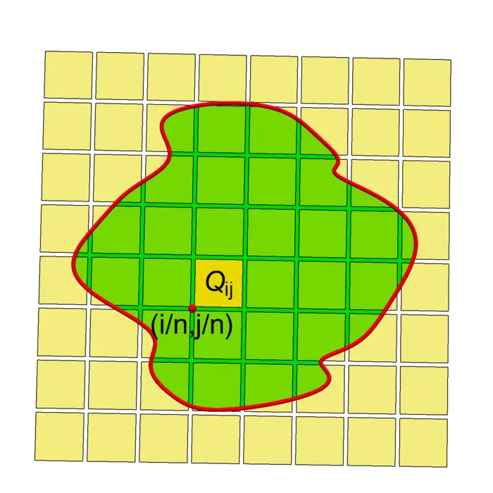
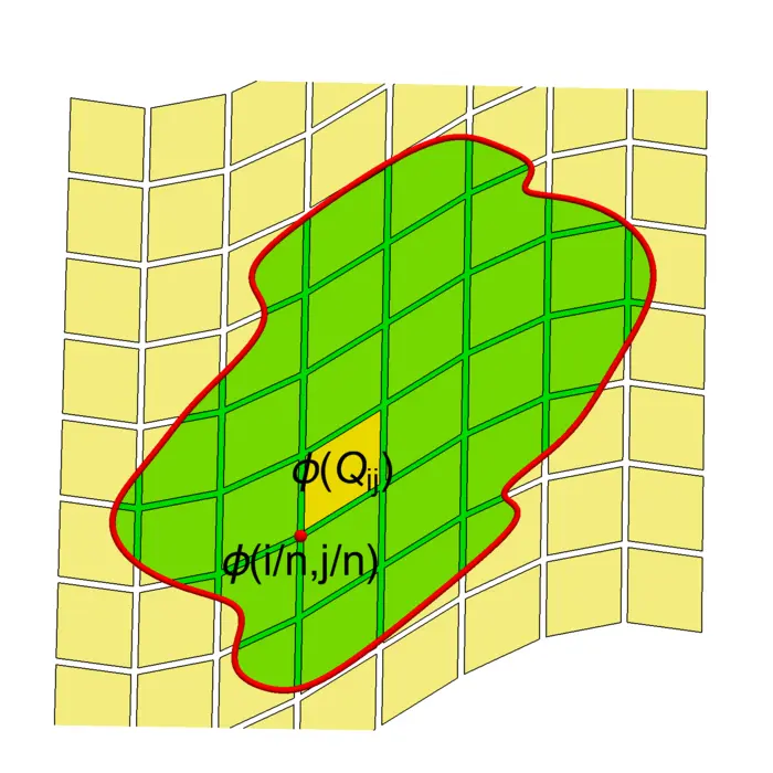
Proof. Cover \(S\) with cubes \(Q_{i j}\) as in the last lecture. Then \[\iint_{S} f(x, y) \,d x \,d y=\sum_{Q_{i j}} \iint_{Q_{i j} \cap S} f(x, y) \,d x \,d y \sim \sum_{i, j} f\Big(\frac{i}{n}, \frac{j}{n}\Big) \frac{1}{n^{2}}.\] The transformed squares \(\Phi(Q_{i j})\) are close to the parallelograms \(d \Phi(Q_{i j})\) which have area \(|d \Phi(i / n, j / n)| / n^{2}\). Now make a quadratic Taylor expansion \[\begin{aligned} \Phi(x, y)=\Phi(x_{0}, y_{0})+d \Phi(x_{0}, y_{0})(x-x_{0}, y-y_{0})+d^{2} \Phi(x_{0}, y_{0})(x-x_{0}, y-y_{0})^{2} / 2 \end{aligned}\] at \((x_{0}, y_{0})=(i / n, j / n)\), where \[\big|d^{2} \Phi(x_{0}, y_{0})(x-x_{0}, y-y_{0})^{2}\big| \leq M_{n}.\] Let \(F=\max _{(x, y) \in R}(|f(x, y)|)\). Applying in every direction, Taylor with remainder, we see \[\left|\int_{\Phi(Q_{i j} \cap S)} f(x, y) \,d x \,d y-f\Big(\Phi\big(\frac{i}{n}, \frac{j}{n}\big)\Big)\right|\, d \Phi\big(\frac{i}{n}, \frac{j}{n}\big)\,\Big|\frac{1}{n^{2}}\Big| \leq \frac{M_{n} F}{n^{2}}\] As the number of squares hitting \(R\) is bound by \(A n^{2}+4 L n\) where \(A\) is the area of \(R\) and \(L\) is the length of the boundary of \(R\), the sum of the non-linear errors is therefore bound by \((A n^{2}+4 L n) \,M_{n} F / n^{2}\) which goes to zero for \(n \rightarrow \infty\). ◻
23.2.2 Integrating a Disk with Change of Variables
Here is an example: If \[\Phi: R=[0,1] \times[0,2 \pi] \rightarrow S=\left\{x^{2}+y^{2} \leq 1\right\}\] is given by \(\Phi(r, \theta)=[r \cos (\theta), r \sin (\theta)]^{T}\), Then \(d \Phi(r, \theta)=r\). If \(f(x, y)=x^{2}+y^{2}=r^{2}\), then \[\iint_{R} r^{2} r \,d r \,d \theta=\iint_{S} (x^{2}+y^{2}) \,d x \,d y.\] The first integral is \(2 \pi / 4\).
23.2.3 Reversing Orientation
Let \(\Phi:[0,1] \times[0,1] \rightarrow[0,1] \times[0,1]\) be given as \(\Phi(x, y)=(y, x)\). Now \(\operatorname{det}(d \Phi)= -1\) and \(|d \Phi|=1\). While we usually could ignore talking about orientation, it is evident here that the integrals considered so far, we do not care about the orientation of the space. If the change of coordinates switches the orientation, the resulting integral does not change.
23.2.4 Coordinate Changes and Elliptical Area Integrals
The chain rule assures that combining two coordinate changes \(\Phi\), \(\Psi\), gives a new coordinate change with \[d(\Psi \circ \Phi)(x)=d \Psi(\Phi(x)) d \Phi(x).\] For example if \(\Psi(x, y)=[a x, b y]^{T}\) and \(\Phi(r, \theta)=[r \cos (\theta), r \sin (\theta)]^{T}\) changes into polar coordinates, then \(\Psi(\Phi(r, \theta))=[ar \cos (\theta), b r \sin (\theta)]^{T}\). Now the image of \(R=[0,1] \times[0,2 \pi]\) is the ellipse \(S=\left\{x^{2} / a^{2}+y^{2} / b^{2} \leq 1\right\}\) and the area of the ellipse is \[A=\iint_{R} a b r \,d r \,d \theta\] because \(\operatorname{det}(d \Phi)=r\) and \(\operatorname{det}(d \Psi)=a b\). The result is \[\int_{0}^{1} \int_{0}^{2 \pi} a b r \,d \theta \,d r=\pi a b.\]
23.2.5 Unveiling Surface Area with Parametrization
Preview: We will next week look at more general cases like \(r: R \subset \mathbb{R}^{2} \rightarrow \mathbb{R}^{3}\) of a parametrized surface, where the distortion factor is \[|d r|=\sqrt{\operatorname{det}(d r^{T} d r)}=|r_{u} \times r_{v}|\] and the surface area is \(\iint_{R}|r_{u} \times r_{v}| \,d u \,d v=\iint_{S} 1 \,d A\).
23.2.6 Change of Variables and Substitution
The theorem generalizes substitution \[\int_{c}^{d} f(\Phi(x))|\Phi^{\prime}(x)| \,d x=\int_{a}^{b} f(x) \,d x\] if \(\Phi(c)=a\) and \(\Phi(d)=b\). We usually insist that \(\Phi\) is monotonically increasing and write \(u=\Phi(x)\), \(d u=\Phi^{\prime}(x) \,d x\) to get computations like in \[\int_{0}^{\sqrt{\pi / 2}} \sin (x^{2}) 2 x \,d x=\int_{0}^{\pi / 2} \sin (u) \,d u,\] where \(\Phi(x)=x^{2}\). As a hack, one can extend the formula to the case when \(\Phi\) can decrease in which case the \([a, b]\) interval becomes the negative \([b, a]\) interval with \(a
Example: Let \(\Phi(x)=2-2 x\) which has \(\Phi^{\prime}=-2\), then \[\int_{1 / 2}^{1}(2-2 x)^{2}|(-2)| \,d x=\int_{0}^{1} x^{2} \,d x.\] In single variable calculus, one can also work with the negative sign case and compute \(\int_{1}^{1 / 2}(2-2 x)^{2}(-2) \,d x\) which works if \(\int_{1}^{1 / 2}=-\int_{1 / 2}^{1}\) but this is not compatible with the defined Riemann integral: we use "spread-sheet" summation and do not distinguish whether we add up the function values from left to right or from right to left.
23.2.7 Fubini and Changing the Order of Integration
We can again look at the Fubini counter example \[\iint_{x^{2}+y^{2} \leq 1} \frac{x^{2}-y^{2}}{(x^{2}+y^{2})^{2}} \,d x \,d y=\int_{0}^{1} \int_{0}^{2 \pi} \frac{\cos (2 \theta)}{r} \,d \theta \,d r=0.\] We can not change the order of integration as we can not integrate \(\int_{0}^{1} 1 / r \,d r\). The trouble also continues in the new coordinate system and it is even more dramatic.
23.2.8 From Chain Rule to Matrix Products
If \(\Phi: x \rightarrow A x\) and \(\Psi: x \rightarrow B x\) are two linear coordinate changes then \(\Psi \circ \Phi=B A\) is the matrix product and the chain rule tells \(|d(\Psi \circ \Phi)|=|\operatorname{det}(A B)|\) which agrees with the product \(|d \Psi||d \Phi|=|\operatorname{det}(A)||\operatorname{det}(B)|\). We can do the verification of the Cauchy-Binet formula \(\operatorname{det}(A B)=\operatorname{det}(A) \operatorname{det}(B)\) directly. If \[A=\left[\begin{array}{ll}a & b \\ c & d\end{array}\right] \quad \text{and} \quad B=\left[\begin{array}{ll}p & q \\ r & s\end{array}\right],\] then \[A B=\left[\begin{array}{ll}a p+b r & a q+b s \\ c p+d r & c q+d s\end{array}\right]\] and you can check the determinant formula.
23.2.9 Open Problem: Inverses of Polynomial Coordinate Changes
Here is a famous open problem about coordinate changes. It is called the Jacobian conjecture. It deals with polynomial coordinate changes, where \(x(u, v)\) and \(y(u, v)\) are polynomials in \(u\), \(v\).
Conjecture: If \(\Phi\) is polynomial and \(|d \Phi|\) is constant different from zero, then \(\Phi\) has a polynomial inverse.
One knows that if the conjecture is false, then there exists a counter example with integer polynomials and Jacobian determinant \(1\). The conjecture is open since at least 1939. An example of a coordinate transformation with determinant \(1\) and integer polynomials are Hénon maps from lecture 16. If \[\Phi([u, v]^{T})=[x, y]^{T}=[u^{2}-u^{4}-v, u]^{T},\] then \[\Phi^{-1}([x, y]^{T})=[y, y^{2}-y^{4}-x]^{T}.\]
23.3 EXAMPLES
Example 1. Problem: What is the area of the image \(S=\Phi(R)\) if \[\Phi([u, v])=[u^{2}-v^{2}+1,2 u v+2]^{T}\] and \(R=\{1 \leq u \leq 3,\ 0 \leq v \leq 1\}\)? (This is \(\Phi(z)=z^{2}+c\) with \(c=1+2 i\) in the complex).
Solution: We have \[d \Phi(u, v)=\left[\begin{array}{cc}2 u & -2 v \\ 2 v & 2 u\end{array}\right]\] and \(|d \Phi(u, v)|=4 u^{2}+4 v^{2}\). We see from the change of variables formula that the area is \[\int_{0}^{1} \int_{1}^{3} (4 u^{2}+4 v^{2}) \,d u \,d v=112 / 3.\]
Example 2. Problem: What is the moment of inertia \(\iint_{R} (x^{2}+y^{2}) \,d x \,d y\), where \(R\) is the polar region given in polar coordinates as \(r \leq 2+\sin (3 \theta)\).
Solution: using the polar coordinate change of variables \(\Phi\) with \(|d \Phi|=r\), we get \[\int_{0}^{2 \pi} \int_{0}^{2+\sin (3 \theta)} r^{2} r \,d r \,d \theta=\int_{0}^{2 \pi}(2+\sin (3 \theta))^{4} / 4 \,d \theta.\] We explain in class how to get the answer \(227 \pi / 4\) quickly.
Example 3. Problem: Here is a famous problem. It is so popular, that it even made it to Hollywood: compute \(\iint_{\mathbb{R}^{2}} e^{-x^{2}-y^{2}} \,d x \,d y\).
Solution: this problem looks difficult at first as we can not integrate with respect to \(x\) or \(y\). The function \(e^{-x^{2}}\) has no elementary anti-derivative. This improper integral is doable in polar coordinates as it is \[\int_{0}^{2 \pi} \int_{0}^{\infty} e^{-r^{2}} r \,d r \,d \theta=\pi.\] It is the inner part \(\int_{0}^{\infty} e^{-r^{2}} r \,d r\) which is an improper integral. One deals with this by approximation. For every finite \(L\) we have \[\int_{0}^{L} e^{-r^{2}} r \,d r=-e^{-r^{2}} /2\Big|_{0}^{L}=1 / 2-e^{-L^{2}} / 2.\] This converges nicely to \(1 / 2\) for \(L \rightarrow \infty\). It follows (and that is the punch line) that \(\int_{-\infty}^{\infty} e^{-x^{2}} \,d x=\sqrt{\pi}\).
EXERCISES
Exercise 1. Given a disk \(R=\left\{x^{2}+y^{2} \leq 1\right\}\), we can make this into a probability space and define the expectation of a function \(f\) as \[\mathrm{E}[f]=\iint_{R} f \,d x \,d y / \pi.\] The expectation of the random variables \(f(x, y)=x^{n}\) are examples of moments. Find \(\mathrm{E}[x]\), \(\mathrm{E}[x^{2}]\), \(\mathrm{E}[x^{3}]\) and \(\mathrm{E}[x^{4}]\).
Exercise 2. What is the volume of the solid bound by \(z=f(x, y)=\) \(x^{2}+y^{2}\) and \(z=g(x, y)=8-x^{2}-y^{2}\) ? You can write this as a double integral \[\iint_{R} \big(g(x, y)-f(x, y)\big) \,d x \,d y\] over a suitable region.
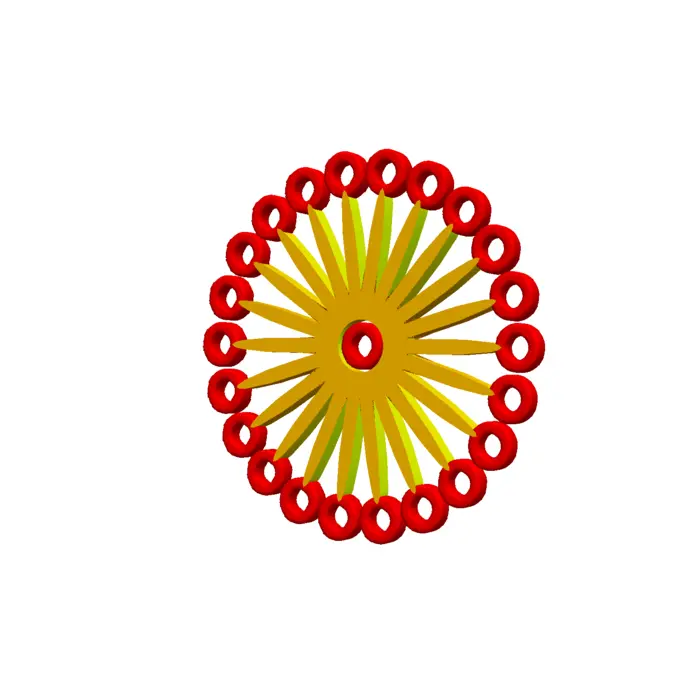
Exercise 3. The fidget spinner is so "\(2017\)" now. What is hot now is the math \(\boldsymbol{22}\) spinner with \(23\) bearings! What is the moment of inertia \(\iint_{G} (x^{2}+y^{2}) \,d x \,d y\) of the math \(\boldsymbol{22}\) fidget spinner region \(G\) given in polar coordinates as \(1 / 2 \leq r \leq 2+\cos (22 \theta)\). To keep our bearings, we do not count the bearings.
Exercise 4. Biologist Piet Gielis once patented polar regions in order to use them to describe biological shapes like cells, leaves, starfish or butterflies. Don’t worry about violating patent laws when finding the area of the following butterfly \[r(t) \leq \big|8-\sin (t)+2 \sin (3 t)+2 \sin (5 t)-\sin (7 t)+3 \cos (2 t)-2 \cos (4 t)\big|.\] (It can produce butterflies in your stomach but there are some tricks to do that fast. Relax with the Math \(22\) fidget spinner for example!)
Exercise 5.
- Prove the Jacobian conjecture for linear maps \(\Phi(x)=A x\), where \(A\) is a \(2 \times 2\) matrix.
- Find a linear coordinate change \(\Phi(x, y)\) for which the Jacobian determinant is \(1\). It should be non-trivial in the sense, that we don’t just want a diagonal matrix \(d \Phi\).
- Find a counter example of the Jacobian conjecture for cubic polynomials (just kidding). Find an example for the Jacobian conjecture where both polynomials are not linear!
- For the \(C^{1}\) case, see J. Schwartz, Mathematical Monthly 61, 1954, or P.D. Lax, Monthly 108, 2001.↩︎