Stokes' Theorem
Table of Contents
32.1 INTRODUCTION
32.1.1 Stokes Theorem
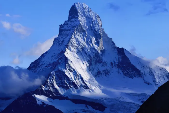
Stokes theorem is a mountain peak in mathematics. You have not really lived before having climbed that mountain. The theorem was developed first in a physics context but it is important for other reasons. First, it is a place where many multi-variable concepts come together: it involves curves, surfaces, the dot and cross products, various derivatives like Jacobean or gradient, integrals or coordinate changes. If you master this theorem you own the bulk of this course. The theorem is also a prototype for a method in science: a theorem helps to solve problems which otherwise would be inaccessible. We will see quite many integrals which are not reachable without the theorem. Also, like mountain climbing, it produces some satisfaction top-out on something that important. The theorem is also beautiful and so art.
32.1.2 Stokes’ Legacy: The Maxwell Equations
Proving the theorem was an exam problem given by George Stokes. James Clerk Maxwell who was a student there would later use it to formulate the Maxwell equations \[\fbox{$d F=0, d^{*} F=j$}\] for the electromagnetic field \(F\) and charge-current \(j\). When space-time \(\mathbb{R}^{4}\) is split into space and time, there are \(4\) equations. One of them is \(\operatorname{curl}(E)=-\frac{\partial}{\partial t} B / c\). It explains how an electric potential \(\int_{C} E \,d r\) emerges from flux changes of a magnetic field \(B\) when turning a wire \(C\), allowing us to generate electricity from motion. When reversed, it turns electricity back into mechanical energy. Think about Stokes theorem next time you are using an electric motor!
32.2 LECTURE
32.2.1 Unveiling the Power of Stokes’ Theorem: Applications and Beauty
Given a \(C^{1}\) surface \(S=r(G)\) in \(\mathbb{R}^{3}\) using a parametrization \(r=[x, y, z]\) and a \(C^{1}\) vector field \(F=[P, Q, R]\), we can form the flux integral \[\iint_{S} F \cdot d S=\iint_{G} F(r(u, v)) \cdot (r_{u} \times r_{v}) \,d u \,d v.\] For \(F=[P, Q, R]\), the curl is defined as \[\nabla \times F=[R_{y}-Q_{z}, P_{z}-R_{x}, Q_{x}-P_{y}].\] The Stokes theorem tells that if \(C=r(I)\) is the boundary of \(S=r(G)\) and \(I\) is oriented so that \(G\) is to the left of \(C\), then
Theorem 1. \(\iint_{S} \operatorname{curl}(F) \cdot d S=\int_{C} F \cdot d r\).
Proof. The key is the following "important formula" \[\operatorname{curl}(F)(r(u, v)) \cdot\left(r_{u} \times r_{v}\right)=F_{u} \cdot r_{v}-F_{v} \cdot r_{u}.\] This is straightforward and done in class. Now define the field \[\tilde{F}(u, v)=[\tilde{P}, \tilde{Q}]=\big[F(r(u, v)) \cdot r_{u}(u, v), F(r(u, v)) \cdot r_{v}(u, v)\big]\] in the \(u v\)-plane. The \(2\)-dimensional curl of \(\tilde{F}\) is \[\tilde{Q}_{u}-\tilde{P}_{v}=F_{u} \cdot r_{v}-F_{v} \cdot r_{u}\] as we can see by using Clairaut \(r_{u v}=r_{v u}\). The Stokes theorem is now a direct consequence of Green’s theorem proven last time.1 ◻
32.3 EXAMPLES
Example 1. Problem: Compute the flux of \(F(x, y, z)=[0,0,8 z^{2}]^{T}\) through the upper half unit sphere \(S\) oriented outwards.
Solution: we parametrize the surface as \[r(u, v)=[\cos (u) \sin (v), \sin (u) \sin (v), \cos (v)]^{T}.\] Because \(r_{u} \times r_{v}=-\sin (v) r\), this parametrization has the wrong orientation! We continue nevertheless and just change the sign at the end. We have \(F(r(u, v))=[0,0,8 \cos ^{2}(v)]^{T}\) so that \[\int_{0}^{2 \pi} \int_{0}^{\pi / 2}-[0,0,8 \cos ^{2}(v)]^{T} \cdot[\cos (u) \sin ^{2}(v), \sin (u) \sin ^{2}(v), \cos (v) \sin (v)]^{T} \,d v \,d u\] The flux integral is \[\int_{0}^{2 \pi} \int_{0}^{\pi / 2} -8 \cos ^{3}(v) \sin (v) \,d v \,d u\] which is \[2 \pi \cdot 8 \cos ^{4}(v)/4 \, \Big|_{0} ^{\pi / 2}=-4 \pi.\] The flux with the outward orientation is \(+4 \pi\). We could not use the Stokes theorem here because we don’t deal with the flux of the curl but the flux of \(F\) itself.
Example 2. Problem: What is the value of \(\int_{C} F \cdot d r\) if \[F=\big[\sin (\sin (x))+z^{2}, e^{y}+x^{3}+y^{2}, \sin (y^{2})+z^{2}\big]\] and \(C\) is the unit polygon \[(0,0,0) \rightarrow (1,0,0) \rightarrow (1,1,0) \rightarrow (0,1,0) \rightarrow (0,0,0)?\] Solution: Use Stokes theorem. The curl of \(F\) is \([2 y \cos (y^{2}), 2 z, 3 x^{2}]\). The surface \(S: r(u, v)=[u, v, 0]\) with \(0 \leq u \leq 1\) and \(0 \leq v \leq 1\) has \(C\) as boundary. Stokes allows to compute \(\iint_{S} \operatorname{curl}(F) \cdot d S\) instead. Since \(r_{u} \times r_{v}=[0,0,1]\), the flux integral is \[\int_{0}^{1} \int_{0}^{1} 3 u^{2} \,d v \,d u=1.\] The computation of the line integral would have been more painful.
Example 3. Problem: Compute the flux of the curl of \(F(x, y, z)=[0,1,8 z^{2}]^{T}\) through the upper half sphere \(S\) oriented outwards.
Solution: Great, it is here, where we can use Stokes theorem \[\iint_{S} \operatorname{curl}(F) \cdot d S=\int_{C} F \cdot d r,\] where \(C\) is the boundary curve which can be parametrized by \(r(t)=[\cos (t), \sin (t), 0]^{T}\) with \(0 \leq t \leq 2 \pi\). Before diving into the computation of the line integral, it is good to check, whether the vector field is a gradient field. Indeed, we see that \(\operatorname{curl}(F)=[0,0,0]\). This means that \(F=\nabla f\) for some potential \(f\) implying by the fundamental theorem of line integrals that \(\int_{C} F \cdot d r=0\). But wait a minute, if the curl of \(F\) is zero, couldn’t we just have seen directly that the flux of the curl through the surface is zero? Yes, we could have seen that before: for a gradient field, the flux of the curl of \(F\) through a surface is always zero, for the simple reason that the curl of such a field is zero.
Example 4. Problem: What is the flux of the curl of \[F(x, y, z)=\big[\sin (x y z), z e^{\cos (x+y)}, z x^{5}+z^{22}\big]\] through the lower ellipsoid \(S\) given by \(x^{2} / 4+y^{2} / 9+z^{2} / 16=1\), \(z<0\)?
Solution: By Stokes theorem, it is the line integral \(\int_{C} F \cdot d r\). Through the boundary \(r(t)=[2 \cos (t), 3 \sin (t), 0]\). But in the \(x y\)-plane \(z=0\), the field \(F\) is zero. The result is zero.
Example 5. Problem: What is the flux of the curl of \(F\) through an ellipsoid \(x^{2} / 4+y^{2} / 9+\) \(z^{2} / 16=1\)?
Solution: We can cut the ellipsoid into two parts to get two surfaces with boundary. The upper part \(S_{+}=\{(x, y, z) \in S,\ z>0\}\) has the boundary \(C_{+}: r(t)=\) \([2 \cos (t), 3 \sin (t), 0]\) which matches the orientation of the surface. Stokes theorem tells that \[\iint_{S_{+}} \operatorname{curl}(F) \cdot d S=\int_{C_{+}} F \cdot d r.\] The lower part \(S_{-}=\{(x, y, z) \in S,\ z<0\}\) has the boundary \(C_{-}: r(t)=[2 \cos (t),-3 \sin (t), 0]\) which matches the orientation of the lower part. Stokes theorem tells that \[\iint_{S_{-}} \operatorname{curl}(F) \cdot d S=\int_{C_{-}} F \cdot d r.\] Together we have \[\int_{C_{-}} F \cdot d r+\int_{C_{+}} F \cdot d r=0\] as the line integrals have just different signs. The result is zero.
32.4 REMARKS
32.4.1 Stokes Theorem in Higher Dimensions
The left hand side of the important formula (it "imports" the curl)2 is defined only in three dimensions. But the right hand side also makes sense in \(\mathbb{R}^{n}\). It is \(\operatorname{tr}((d F)^{*} d r)\), where \(*\) rotates the \(2\)-frame by \(90\) degrees. The Stokes theorem for \(2\)-surfaces works for \(\mathbb{R}^{n}\) if \(n \geq 2\). For \(n=2\), we have with \(x(u, v)=u\), \(y(u, v)=v\) the identity \[\operatorname{tr}((d F)^{*} d r)=Q_{x}-P_{y}\] which is Green’s theorem. Stokes has the general structure , where \(\delta F\) is a derivative of \(F\) and \(\delta G\) is the boundary of \(G\).
Theorem 2. Stokes holds for fields \(F\) and \(2\)-dimensional \(S\) in \(\mathbb{R}^{n}\) for \(n \geq 2\).
32.4.2 Integral Theorems: Simplifying Statistics in High Dimensions
Why are we interested in \(\mathbb{R}^{n}\) and not only in \(\mathbb{R}^{3}\)? One example is that \(2\)-dimensional surfaces appear as "paths" which a moving string in \(11\) dimension traces. More important maybe is that statisticians work by definition in high dimensional spaces. When dealing with \(n\) data points, one works in \(\mathbb{R}^{n}\). Why would you care about theorems like Stokes in statistics? As a matter of fact, integral theorems in general allow to simplify computations. As we have seen in Green’s theorem, when computing the sum over all the curls, there are cancellations happening in the inside. Integral theorems "see these cancellations" and allow to bypass and ignore stuff which does not matter.
32.4.3 Generalizing Line Integrals and Flux Integrals: Beyond the Cross Product
The fundamental theorem of line integrals \[\int_{a}^{b} \operatorname{tr}(d f(r(t)) d r(t)) \,d t=f(r(b))-f(r(a))\] holds also in \(\mathbb{R}^{n}\). The flux integral \[\iint_{G} \operatorname{tr}(F^{*}(r(u, v)) \,d r(u, v)) \,d u \,d v\] is the analogue of a line integral in two dimensions. Written like this, we don’t need the cross product. And not yet the language of differential forms.
32.4.4 Stokes Theorem, Geometry, and Minimization
Stokes deals with "fields" and "space". What happens if the field is space itself, that is if \(F^{*}=d r\)? It is of interest. For \(m=1\), and \(F=d r^{T}\), then \(\int_{a}^{b}|d r|^{2} \,d t\) is the action integral in physics. A general Maupertius principle assures that it is equivalent to the arc length \(\int_{a}^{b}|d r| \,d t\) in the sense that minimizing arc length between two points is equivalent to minimize the action integral (which is more like the energy one uses to get from the first point to the second). Now, in two dimensions we have \[\iint_{G} \operatorname{tr}(d r^{T} d r) \,d u \,d v.\] We can compare this with \[\iint_{G} \operatorname{det}(d r^{T} d r) \,d u \,d v\] which is called the Nambu-Goto action, which resembles the surface area \[\iint_{G} \sqrt{\operatorname{det}(d r^{T} d r)} \,d u \,d v\] also called the Polyakov action. Nature likes to minimize. Free particles move on shortest paths, minimize the arc length. Maupertius tells that minimizing the length \(\int_{A}^{B}|r^{\prime}(t)| \,d t\) of a path equivalent to minimizing \(\int_{A}^{B} r^{\prime}(t) \cdot r^{\prime}(t) \,d t\) which essentially is the integrated kinetic energy or gasoline use to go from \(A\) to \(B\). For the purpose of minimizing stuff this also works for two dimensional actions. Minimizing the surface area \(\iint_{G}|r_{u} \times r_{v}| \,d u \,d v\) among all surfaces connecting two one dimensional curves is equivalent to minimize \(\iint_{G}|r_{u} \times r_{v}|^{2} \,d u \,d v\). Also in higher dimensions, Nambu-Goto and Polyakov are equivalent.
EXERCISES
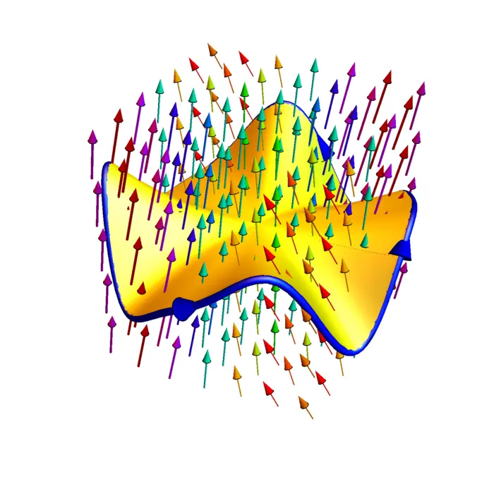
Exercise 1. Use Stokes to find \(\int_{C} F \cdot d r\), where \[F(x, y, z)=\big[12 x^{2} y, 4 x^{3}, 12 x y+e^{(e^{z})}\big]\] and \(C\) is the curve of intersection of the hyperbolic paraboloid \(z=y^{2}-x^{2}\) and the cylinder \(x^{2}+y^{2}=1\), oriented counterclockwise as viewed from above.
Exercise 2. Evaluate the flux integral \(\iint_{S} \operatorname{curl}(F) \cdot d S\), where \[F(x, y, z)=\Big[x e^{y^{2}} z^{3}+2 x y z e^{x^{2}+z}, x+z^{2} e^{x^{2}+z}, y e^{x^{2}+z}+z e^{x}\Big]^{T}\] and where \(S\) is the part of the ellipsoid \(x^{2}+y^{2} / 4+(z+1)^{2}=2\), \(z>0\) oriented so that the normal vector points upwards.
Exercise 3. Find the line integral \(\int_{C} F \,d r\), where \(C\) is the circle of radius \(3\) in the \(x z\)-plane oriented counter clockwise when looking from the point \((0,1,0)\) onto the plane and where \(F\) is the vector field \[F(x, y, z)=\big[4 x^{2} z+x^{5}, \cos (e^{y}),-4 x z^{2}+\sin (\sin (z))\big]^{T}.\] Use a convenient surface \(S\) which has \(C\) as a boundary.
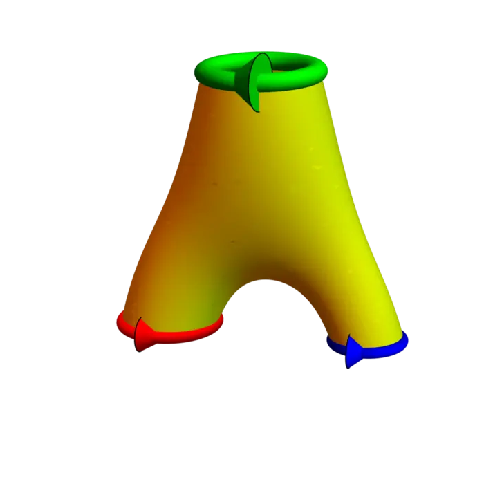
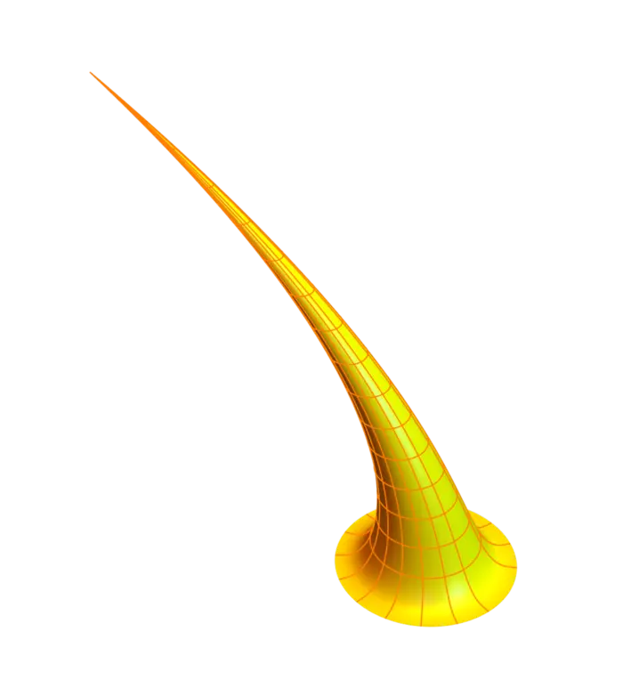
Exercise 4. Find the flux integral \(\iint_{S} \operatorname{curl}(F) \cdot d S\), where \[F(x, y, z)=\Big[y+2 \cos (\pi y) e^{2 x}+z^{2}, x^{2} \cos (z \pi / 2)-\pi \sin (\pi y) e^{2 x}, 2 x z+(z-1)^{22}\Big]^{T}\] and \(S\) is the surface parametrized by \[r(s, t)=\big[(1-s^{1 / 3}) \cos (t)-4 s^{2},(1-s^{1 / 3}) \sin (t), 5 s\big]^{T}\] with \(0 \leq t \leq 2 \pi\), \(0 \leq s \leq 1\) and oriented so that the normal vectors point to the outside of the thorn.
Exercise 5. Assume \(S\) is the surface \(x^{22}+y^{8}+z^{6}=100\) and \[F=\big[e^{e^{22 z}}, 22 x^{2} y z, x-y-\sin (z x)\big].\] Explain why \(\iint_{S} \operatorname{curl}(F) \cdot d S=0\).
Appendix: Applications
32.4.5 Simply Connected Regions and Conservative Fields
A region \(E\) in \(\mathbb{R}^{n}\) is called simply connected if it is connected and for every closed loop \(C\) in \(E\) there is a continuous deformation \(C_{s}\) of \(C\) within \(G\) such that \(C_{0}=C\) and \(C_{1}(t)=P\) is a point. For example, \(C(t)=[\cos (t), \sin (t), 0]\) can be deformed in \(E=\mathbb{R}^{3}\) to a point with \[C_{s}(t)=[(1-s) \cos (t),(1-s) \sin (t), 0]\] as \(C_{1}(t)=P=[0,0,0]\) for all \(t\). Each Euclidean space \(\mathbb{R}^{n}\) is simply connected. The region \(G=\{x^{2}+y^{2}>0\} \subset \mathbb{R}^{3}\) is not simply connected as the circle \(C: r(t)=[\cos (t), \sin (t), 0]\) winding around the \(z\)-axis can not be pulled together to a point within \(G\). The region \(G=\{x^{2}+y^{2}+z^{2}>0\} \subset \mathbb{R}^{3}\) is simply connected, but \(G=\{x^{2}+y^{2}>0\}\) in \(\mathbb{R}^{2}\) is not. Remember that \(F\) was called irrotational if \(\operatorname{curl}(F)=0\) everywhere.
Theorem 3. If \(F\) is irrotational on a simply connected \(E\) then \(F=\nabla f\) in \(E\).
Proof. Since \(E\) is simply connected and \(\operatorname{curl}(F)=0\), every closed loop \(C\) can be filled in by a surface \(S=\bigcup_{0 \leq s \leq 1} C_{s}\) which has the boundary \(C\). Stokes theorem gives \[\int_{S} F \cdot d r=\iint_{S} \operatorname{curl}(F) \cdot d S=0.\] The closed loop property implies path independence. A potential \(f\) can be obtained by fixing a base point \(p\) in \(E\), then define for any other point \(x\) a path \(C_{p x}\) going from \(p\) to \(x\). The potential function \(f\) is then defined as \(f(x)=\int_{C_{p x}} F \cdot d r\). ◻
32.4.6 Non-Simply Connected Domains and Conservative Fields
The field \[F(x, y, z)=\big[-y /(x^{2}+y^{2}), x /(x^{2}+y^{2}), 0\big]\] is defined everywhere except on the \(z\)-axis. The domain \(E\), where \(F\) is defined is not simply connected. There is no global function \(f\) which is a potential for \(F\).
32.4.7 Simply Connectedness in Topology
The notion of "simply connectedness" is important in topology. The first solved Millenium problem, the Poincaré conjecture, is now a theorem. It tells that a \(3\)-dimensional manifold which is simply connected is topologically equivalent to the \(3\)-sphere \[\{x^{2}+y^{2}+z^{2}+w^{2}=1\} \subset \mathbb{R}^{4}.\] In two dimensions, the result was known for a long time already, because the structure of \(2\)-dimensional connected manifolds is known.
ELECTROMAGNETISM
32.4.8 Maxwell-Faraday and Stokes: Generating Electricity from Magnetism
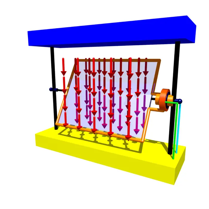
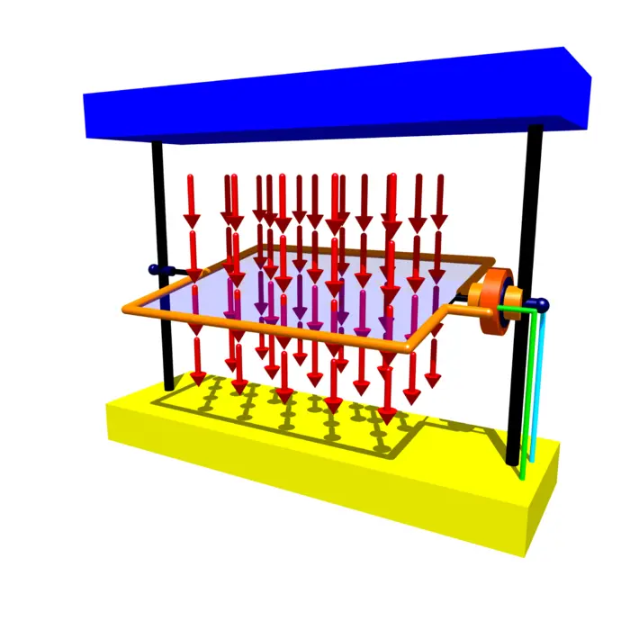
The Maxwell-Faraday equation in electromagnetism relates the electric field \(E\) and the magnetic field \(B\) with the partial differential equation \(\operatorname{curl}(E)=\) \(-\frac{d}{d t} B\). Given a surface \(S\), the flux integral \(\iint_{S} B \cdot d S\) is called the magnetic flux of \(B\) through the surface. If we integrate the Maxwell-Faraday equation, we see that \(\iint_{S} \operatorname{curl}(E) \cdot d S\) is equal to minus the rate of change of the magnetic flux \(-\frac{d}{d t} \iint_{S} B \cdot d S\). Stokes theorem now assures that \(\iint_{S} \operatorname{curl}(E) \cdot d S=\int_{C} E \cdot d r\) is the line integral of the electric field along the boundary. But this is electric potential or voltage. We see:
We can generate an electric potential by changing the magnetic flux.
32.4.9 Flux Changes and Electricity Generation
Changing the magnetic flux can happen in various ways. We can generate a changing magnetic field by using alternating current. This is how transformers work. An other way to change the flux is to rotate a wire in a fixed magnetic field. This is the principle of the dynamo:
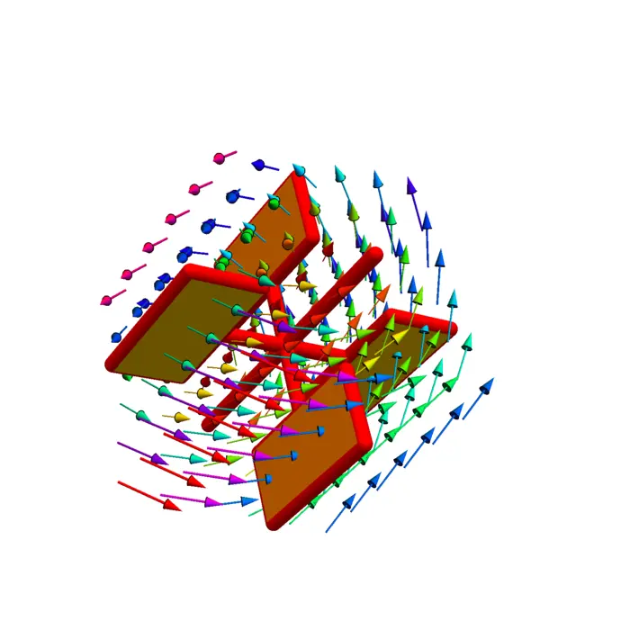
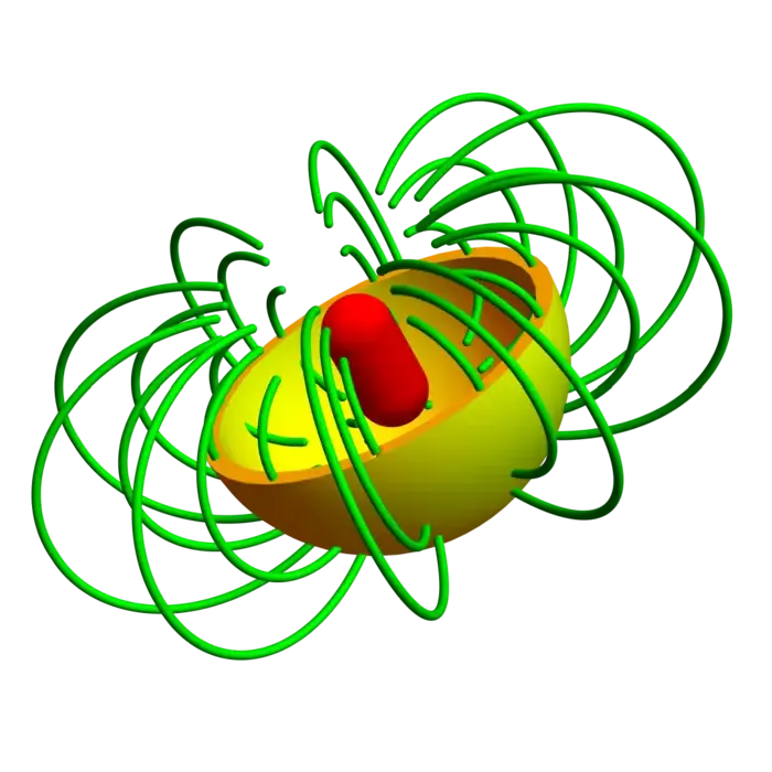
32.4.10 Stokes Theorem and Dipole Flux
The vector field \[A(x, y, z)=\frac{[-y, x, 0]}{(x^{2}+y^{2}+z^{2})^{3 / 2}}\] is called the vector potential of a magnetic field \(B=\operatorname{curl}(A)\). The picture shows some flow lines of this magnetic dipole field \(B\).
Problem: Find the flux of \(B\) through the lower half sphere \(x^{2}+y^{2}+z^{2}=1\), \(z \leq 0\) oriented downwards.
Solution: Since we have an integral of the curl of the vector field \(A\), we use Stokes theorem and integrate \(A(r(t))\) along the boundary curve \(r(t)=[\cos (t),-\sin (t), 0]\). First of all, we have \(A(r(t))=[\sin (t), \cos (t), 0]\). The velocity is \(r^{\prime}(t)=[-\sin (t), \cos (t), 0]\). The integral is \(\int_{0}^{2 \pi} -1 \,d t=-2 \pi\).
32.4.11 E and B: Maxwell’s Equations in a Nutshell
Here are all the four magical Maxwell equations for the electric field \(E\) and magnetic field \(B\) related to the charge density \(\sigma\) and the electric current \(j\). The constant \(c\) is the speed of light. (By using suitable coordinates, one can assume \(c=1\).) \[\fbox{$\operatorname{div}(E)=4 \pi \sigma, \quad \operatorname{div}(B)=0, \quad c \cdot \operatorname{curl}(E)=-B_{t}, \quad c \cdot \operatorname{curl}(B)=E_{t}+4 \pi j.$}\]
FLUID DYNAMICS
32.4.12 Helmholtz’s Theorem
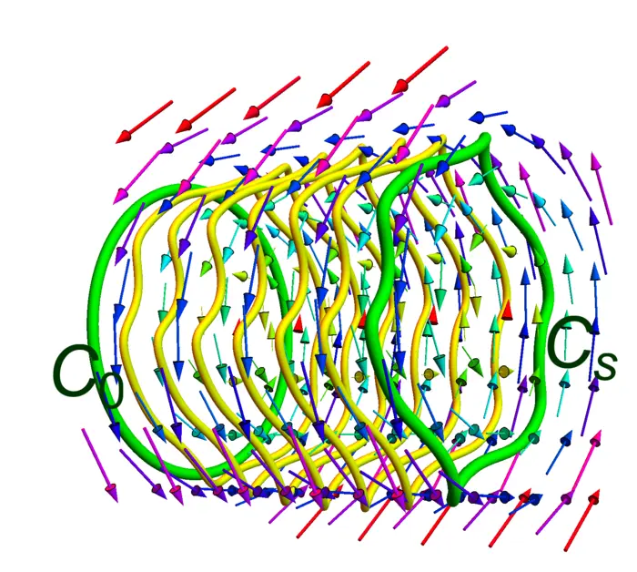
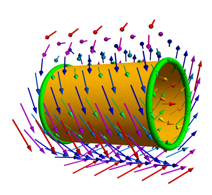
If \(F\) is the fluid velocity field and \(C\) is a closed curve, then \(\int_{C} F \cdot d r\) is called the circulation of \(F\) along \(C\). The curl of \(F\) is called the vorticity of \(F\). A vortex line is a flow line of \(\operatorname{curl}(F)\). Given a curve \(C\), we can let any point in \(C\) flow along the vorticity field. This produces a vortex tube \(S\). The flux of the vorticity though a surface \(S\) is the vortex strength of \(F\) through \(S\). Stokes theorem implies the Helmholtz theorem.
Theorem 4. If \(C_{s}\) flows along \(F\), then \(\int_{C_{s}} F \cdot d r\) stays constant.
Proof. Let \(C\) be a closed curve and \(C_{s}(t)\) be the curve after letting it flow using a deformation parameter \(s\). The deformation produces a tube surface \(S=\bigcup_{s=0}^{t} C_{s}\) which has the boundary \(C\) and \(C_{t}\). Since the curl of \(F\) is always tangent to the surface \(S\), the flux of the curl of \(F\) through \(S\) is zero. Stokes theorem implies that \[\int_{C} F \cdot d r-\int_{C_{s}} F \cdot d r=0.\] The negative sign is because the orientation of \(C_{s}\) is different from the orientation of \(C\) if the surface has to be to the left. ◻
COMPLEX ANALYSIS
32.4.13 Complex Green’s Theorem and Analytic Magic
An application of Green’s theorem is obtained, when integrating in the complex plane \(\mathbb{C}\). Given a function \(f(z)=u(z)+i v(z)\) from \(\mathbb{C} \rightarrow \mathbb{C}\) and a closed path \(C\) parametrized by \(r(t)=x(t)+i y(t)\) in \(\mathbb{C}\), define the complex integral \[\int_{a}^{b} \Big(u\big(x(t)+i y(t)\big)+i v\big(x(t)+i y(t)\big)\Big)\big(x^{\prime}(t)+i y^{\prime}(t)\big) \,d t.\] This is \[\int_{a}^{b} \big(u(r(t)) x^{\prime}(t)-v(r(t)) y^{\prime}(t)\big) \,d t+i \int_{a}^{b} \big(v(r(t)) x^{\prime}(t)+u(r(t))^{\prime}(t)\big) \,d t.\] These are two line integrals. The real part is \(F=\) \([u,-v]\), the imaginary part is \(F=[v, u]\). Assume \(C\) bounds a region \(G\), then Green’s theorem tells that the first integral is \(\iint_{G}(-v_{x}-u_{y}) \,d x \,d y\) and the second integral is \(\iint_{G} (u_{x}-v_{y}) \,d x \,d y\). It turns out now that for nice functions \(f\) like polynomials, the Cauchy-Riemann differential equations hold so that these line integrals are zero. We have therefore:
Theorem 5. If \(f\) is a polynomial and \(C\) a closed loop, \(\int_{C} f(z) \,d z=0\).
- Mathematicians say: "we pulled back the field from \(\mathbb{R}^{3}\) to \(\mathbb{R}^{2}\) along the parametrization".↩︎
- I learned the "important formula" from Andrew Cotton-Clay in 2009: http://www.math.harvard.edu/archive/21a_fall_09/exhibits/stokesgreen↩︎