Pythagorean Theorem
Table of Contents
1.1 INTRODUCTION
1.1.1 Exploring the Pythagorean Theorem: Its History and Significance
In this first lecture, we look at one of the most important theorems in mathematics, the theorem of Pythagoras. The historical roots of the theorem are mesmerizing: the first examples of identities like \(5^{2}+12^{2}=13^{2}\) already appeared in Sumerian mathematics. Triples of numbers like \((5,12,13)\) are called Pythagorean triples. The theorem itself is much more than that. The theorem not only lists a few examples for evidence but states and proves that for all triangles, the relation \(a^{2}+b^{2}=c^{2}\) holds if and only if the triangle is a right angle triangle. Without exaggeration, the Pythagorean theorem is one of the most beautiful and most important theorems. It has cameos in various other parts of mathematics. In harmonic analysis for example, it tells that the square of the length of a periodic function is the sum of the squares of its Fourier coefficients. In probability theory it tells that if two random variables \(X, Y\) are uncorrelated, then the variance of \(X+Y\) is the sum of the variance of \(X\) and \(Y\).
1.1.2 Redefining Vectors
We use here the theorem also while introducing vectors and linear spaces. The language of matrices is not only a matter of notation, but also allows for a slightly more sophisticated approach to vector calculus in which one distinguishes between column vectors and row vectors. Unlike in standard vector analysis courses, this is possible when working closer to linear algebra. Traditionally, many sources define a vector as a quantity with "magnitude" and "direction". This is highly problematic as a "movie" qualifies for this notion: it has a length and has a director. But we don’t need to mock this with a pun: the zero vector \(0\) is a quantity which would not qualify as a vector because the zero vector does not have a direction. Because of such problems, one usually defines a vector as a quantity defined by two points \(A, B\) in space, writes \(\overrightarrow{A B}\) and thinks about the vector as a translation from \(A\) to \(B\) or as an "arrow" starting from \(A\) and ending at \(B\). Now, one has the difficulty that two parallel vectors of equal length are identified. One actually uses equivalence classes to get from affine space to linear space. The modern point of view is that one can attach a linear space of vectors at every point and think of \(\overrightarrow{A B}\) as a vector attached to the point \(A\). We will see for example the concept of a gradient field, which attaches at every point a row vector. Force fields are examples.
1.1.3 Matrix Foundations in Data Analysis
In any case, introducing spaces of matrices early has advantages also in a time where data analysis is recognized as an important tool. Relational data bases are founded on the concept of matrices. Most familiar are spread sheets which are two-dimensional arrays in which data are organized. More recently, such concept are also displaced with more sophisticated data structures like graph data bases. Still, a graph can also be described by matrices. Given two nodes \(x, y\) of the network, write in the matrix entry \(A_{x y}\) tells how they are related. In the simplest case put a \(1\) if the nodes are connected and \(0\) if they are not connected. In any case, data are always arrays of more basic quantities. The memory structure of a computer is organized as an array. As Alan Turing has shown, all computations we have formalized can be done on a one dimensional tape with entries \(0\) and \(1\). Modern computer storage devices are essentially such Turing tapes, but organized in a more sophisticated way, using partitions or sectors similarly as matrices are organized with rows and columns.
1.2 LECTURE
1.2.1 Matrix Essentials
A finite rectangular array \(A\) of real numbers is called a matrix. If there are \(n\) rows and \(m\) columns in \(A\), it is called an \(n \times m\) matrix. We address the entry in the \(i\)’th row and \(j\)’th column with \(A_{i j}\). An \(n \times 1\) matrix is a column vector, a \(1 \times n\) matrix is a row vector. A \(1 \times 1\) matrix is called a scalar. Given an \(n \times p\) matrix \(A\) and a \(p \times m\) matrix \(B\), the \(n \times m\) matrix \(A B\) is defined as \[(A B)_{i j}=\sum_{k=1}^{p} A_{i k} B_{k j}.\] It is called the matrix product. The transpose of an \(n \times m\) matrix \(A\) is the \(m \times n\) matrix \(A_{i j}^{T}=A_{j i}\). The transpose of a column vector is a row vector.
1.2.2 Vector Space of Matrices
Denote by \(M(n, m)\) the set of \(n \times m\) matrices. It contains the zero matrix \(O\) with \(O_{i j}=0\). In the case \(m=1\), it is the zero vector. The addition \(A+B\) of two matrices in \(M(n, m)\) is defined as \[(A+B)_{i j}=A_{i j}+B_{i j}.\] The scalar multiplication \(\lambda A\) is defined as \[(\lambda A)_{i j}=\lambda A_{i j}\] if \(\lambda\) is a real number. These operations make \(M(n, m)\) a vector space \(=\) linear space: the addition is associative, commutative with a unique additive inverse \(-A\) satisfying \[A-A=0.\] The multiplications are distributive: \[A(B+C)=A B+A C\] and \[\lambda(A+B)=\lambda A+\lambda B\] and \[\lambda(\mu A)=(\lambda \mu) A.\]
1.2.3 Euclidean Spaces, Dot Products, and Length
The space \(M(n, 1)\) is also called \(\mathbb{R}^{n}\). It is the \(\boldsymbol{n}\)-dimensional Euclidean space. The vector space \(\mathbb{R}^{2}\) is the plane and \(\mathbb{R}^{3}\) is the physical space. These spaces are dear to us as we draw on paper and live in space. The dot product between two column vectors \(v, w \in \mathbb{R}^{n}\) is the matrix product \[v \cdot w=v^{T} w.\] Because the dot product is a scalar, the product is also called the scalar product. In the matrix product of two matrices \(A, B\), the entry at position \((i, j)\) is the dot product of the \(i\)’th row in \(A\) with the \(j\)’th column in \(B\). More generally, the dot product between two arbitrary \(n \times m\) matrices can be defined by \[A \cdot B=\operatorname{tr}(A^{T} B),\] where the trace of a matrix is the sum of its diagonal entries. This means \[\operatorname{tr}(A^{T} B)=\sum_{i, j} A_{i j} B_{i j}.\] We just take the product over all matrix entries and add them up. The dot product is distributive \[(u+v) \cdot w=u \cdot w+v \cdot w\] and commutative \[v \cdot w=w \cdot v.\] We can use it to define the length \[|v|=\sqrt{v \cdot v}\] of a vector or the length \(|A|\) of a matrix, where we took the positive square root. The sum of the squares is zero exactly if all components are zero. The only vector satisfying \(|v|=0\) is therefore \(v=0\).
1.2.4 Cauchy-Schwarz Inequality
An important key result is the Cauchy-Schwarz inequality.
Theorem 1. \(|v \cdot w| \leq|v||w|\)
Proof. If \(w=0\), there is nothing to prove as both sides are zero. If \(w \neq 0\), then we can divide both sides of the equation by \(|w|\) and so achieve that \(|w|=1\). Define \(a=v \cdot w\). Now, \[\begin{aligned} 0 \leq(v-a w) \cdot(v-a w)&=|v|^{2}-2 a v \cdot w+a^{2}|w|^{2}\\ &=|v|^{2}-2 a^{2}+a^{2}\\ &=|v|^{2}-a^{2} \end{aligned}\] meaning \(a^{2} \leq|v|^{2}\) or \(v \cdot w \leq|v|=|v||w|\). ◻
1.2.5 Angle Between Two Vectors
It follows from the Cauchy-Schwarz inequality that for any two non-zero vectors \(v, w\), the number \((v \cdot w) /(|v||w|)\) is in the closed interval \([-1,1]\): \[-1\leq \frac{u \cdot w}{|v| |w|}\leq 1.\] There exists therefore a unique angle \(\alpha \in[0, \pi]\) such that \[\cos (\alpha)=\frac{v \cdot w}{|v||w|}\] If this angle between \(v\) and \(w\) is equal to \(\alpha=\pi / 2\), the two vectors are orthogonal. If \(\alpha=0\) or \(\pi\) the two vectors are called parallel. There exists then a real number \(\lambda\) such that \(v=\lambda w\). The zero vector is considered both orthogonal as well as parallel to any other vector.
1.2.6 Law of Cosines
Two vectors \(v, w\) define a (possibly degenerate) triangle \(\{0, v, w\}\) in Euclidean space \(\mathbb{R}^{n}\). The above formula defines an angle \(\alpha\) at the point \(0\) (which could be the zero angle). The side lengths \(a=|v|, b=|w|, c=|v-w|\) of the triangle satisfy the following cos formula. It is also called the Al-Kashi identity.
Corollary 1. \[c^{2}=a^{2}+b^{2}-2 a b \cos (\alpha)\]
Proof. We use the definitions as well as the distributive property (FOIL out): \[\begin{aligned} c^{2}&=|v-w|^{2}\\ &=(v-w) \cdot(v-w)\\ &=v \cdot v+w \cdot w-2 v \cdot w\\ &=a^{2}+b^{2}-2 a b \cos (\alpha) \end{aligned}\] ◻
1.2.7 Understanding the Pythagorean Theorem: A Special Case of the Law of Cosines
The case \(\alpha=\pi / 2\) is particularly important. It is the Pythagorean theorem:
Theorem 2. In a right angle triangle we have \(c^{2}=a^{2}+b^{2}\).
1.3 EXAMPLES
Example 1. The dot product \(\left[\begin{array}{l}1 \\ 3 \\ 1\end{array}\right] \cdot\left[\begin{array}{c}1 \\ -2 \\ -1\end{array}\right]\) is \[[1,3,1]\left[\begin{array}{c}1 \\ -2 \\ -1\end{array}\right]=1-6-1=-6.\] We have \(|v|=\sqrt{11},|w|=\sqrt{6}\) and angle \(\alpha=\arccos (-6 / \sqrt{66})\).
Example 2. The dot product of \(A=\left[\begin{array}{ll}3 & 1 \\ 2 & 1\end{array}\right]\) and \(B=\left[\begin{array}{cc}2 & 2 \\ 4 & -1\end{array}\right]\) is \[\operatorname{tr}\left(A^{T} B\right)=6+2+8+(-1)=15.\] The length of \(A\) is \(\sqrt{\operatorname{tr}(A^T A)}=\sqrt{12}\), the length of \(B\) is \(\sqrt{\operatorname{tr}(B^T B)}=5\). The angle between \(A\) and \(B\) is \[\alpha=\arccos \frac{15}{5 \sqrt{12}}=\arccos \frac{\sqrt{3}}{2}=\frac{\pi}{6}.\]
Example 3. \(A=\left[\begin{array}{ll}1 & 2 \\ 1 & 2\end{array}\right]\) and \(B=\left[\begin{array}{cc}1 & -1 \\ -1 & 1\end{array}\right]\) are perpendicular because \[\operatorname{tr}(A^{T} B)=0.\] The angle between them is \(\dfrac{\pi}{2}\). The length of \(A\) is \(a=\sqrt{10}\). The length of \(B\) is \(b=\sqrt{4}=2\). The length of \[A+B=\left[\begin{array}{ll}2 & 1 \\ 0 & 3\end{array}\right]\] is \(c=\sqrt{14}\). We confirm \[a^{2}+b^{2}=c^{2}.\] Note that \(A B \neq B A\). Multiplication is not commutative.
Example 4. Find the angles in a triangle of length \(a=4, b=5\) and \(c=6\).
Answer: Al Kashi gives \[2 \cdot 4 \cdot 5 \cos (\gamma)=4^{2}+5^{2}-6^{2}=5\] so that \[\gamma=\arccos (5 / 40).\] Similarly \(2 \cdot 4 \cdot 6 \cos (\beta)=27\) so that \(\gamma=\arccos (27 / 48)\) and \[2 \cdot 5 \cdot 6 \cos (\alpha)=45\] so that \(\alpha=\arccos (45 / 60).\)
1.4 ILLUSTRATION
1.4.1 Infinite Horizons in Mathematics
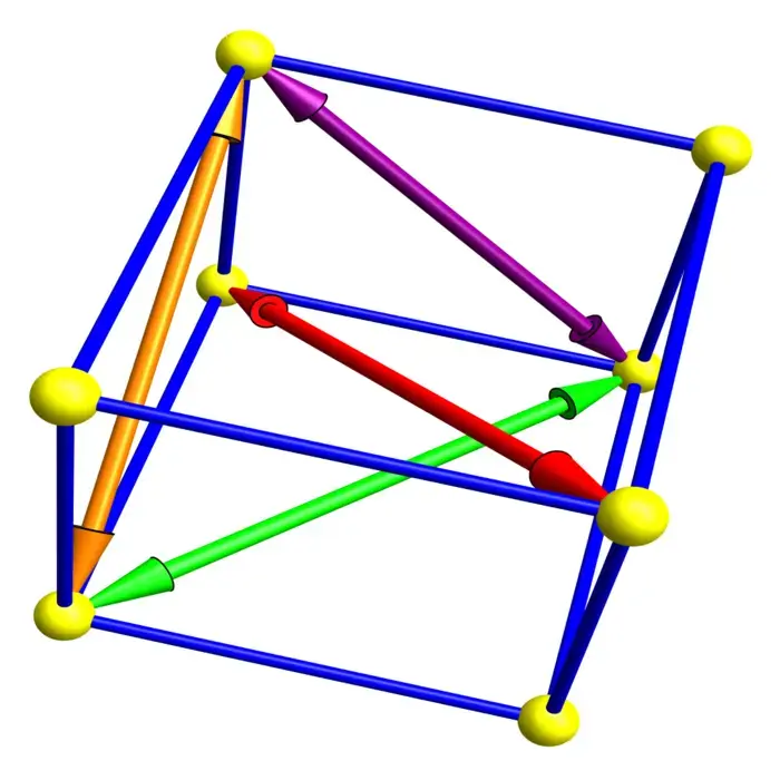
Mathematics is not only eternal, but also infinite. To illustrate this, look at the "Eternals" problem.1 Define the Babylonian graph \(B\) in which the positive integers are the vertices and where \((a, b)\) are connected, if \(a^{2}+b^{2}\) is a perfect square. Every edge in \(B\) belongs to a Pythagorean triple \(a^{2}+b^{2}=c^{2}\). One can ask which type of sub-graphs appear, how many connected components there are, whether the diameter is infinite, or how large closed loops can become. Hundreds of questions could be asked. Embedded triangles \(K_{3}\) in \(B\) for example are Euler bricks! Are there embedded tetrahedra \(K_{4}\), cliques of numbers \((a, b, c, d)\) for which every pair is a Pythagorean triple? This would be an Eulerian tesseract. Is there one? Before proving anything, we have a data problem. Experiment!
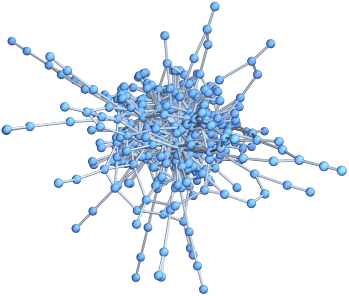
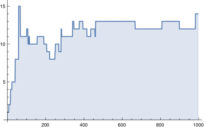
ListPlot[Table[GraphDiameter[Babylonian[n]],n,1000]] gives the diameter of the largest component \(B_{1}(n)\) of \(B(n)\). We have \(\operatorname{Diam}\left(B_{1}(5000)\right)=18, \operatorname{Diam}\left(B_{1}(10000)\right)=29\).EXERCISES
Exercise 1. Use the definitions to find the angle \(\alpha\) between the vector \(v=[1,1,0,-3,2,1]^{T}\) and \(w=[1,1,9,-3,-5,-3]^{T}\) in \(\mathbb{R}^{6}\). If we think about \(v, w\) as data, the value \(\cos (\alpha)\) is the correlation between the two data points \(v\) and \(w\). If the cosine is positive, the data have positive correlation. If the cosine is negative, they have negative correlation.
Exercise 2. Given the matrix \(A=\left[\begin{array}{lll}1 & 2 & 3 \\ 4 & 5 & 6 \\ 7 & 8 & 9\end{array}\right]\).
- Find \(A^{T}\), then build \(B=A+A^{T}\) and \(C=A-A^{T}\). The first matrix is called symmetric, the second is called anti-symmetric.
- Compute \(A A^{T}\) and \(A^{T} A\). Then evaluate \(\operatorname{tr}(A^{T} A)\) and \(\operatorname{tr}(AA^{T})\).
- Why are these two numbers computed in b) the same? Is it true in general for two \(n \times m\) matrices that \(\operatorname{tr}(A^{T}B)=\operatorname{tr}(B^{T}A)\)? (There is a short verification using the sum notation).
Exercise 3.
- Verify the triangle identity \(|v-w| \leq|v|+|w|\) in general by FOILing out \((v-w) \cdot(v-w)\), then generate an example of two vectors with integer coordinates in the plane \(\mathbb{R}^{2}\), where one can apply this. Draw the situation.
- Verify that if \(v\) and \(w\) have the same length, then \((v-w)\) and \((v+w)\) are perpendicular. Describe the situation in b) geometrically in a sentence.
Exercise 4. Write the vector \(F=[2,3,4]^{T}\) as a sum of a vector parallel to \(v=[1,1,1]^{T}\) and a vector perpendicular to \(v\). If we interpret \(F\) as a force acting on a kite of mass \(1\) and \(v\) as the velocity then \(F \cdot v\) has an interpretation as power, the rate of change of the energy of the kite. The vector parallel to \(v\) would by Newton be the acceleration of the kite.
Exercise 5.
- Find two vectors in \(\mathbb{R}^{2}\) for which all coordinate entries are \(1\) or \(-1\) and which are both perpendicular to each other.
- Design four vectors in \(\mathbb{R}^{4}\) for which all coordinate entries are \(1\) or \(-1\) which are all perpendicular to each other.
Optional: can you invent a strategy which allows you for example to find \(16\) vectors in \(\mathbb{R}^{16}\) which are all perpendicular to each other and have still entries in \(\{-1,1\}\)?
- This problem has been communicated to us by Ajak, who knows thousands of years of mathematics↩︎