Parametrization
Table of Contents
11.1 INTRODUCTION
11.1.1 Unwrapping Shapes: The Magic of Parametrization
We have seen that when parametrizing curves \(r(t)\), we have much more control than when looking at curves given by equations. It would be difficult to describe a helix \(r(t)=[\cos (t), \sin (t), t]\) in terms of equations for example. For surfaces also, it is good to have as many coordinates as the dimension. We live on a two dimensional sphere \(x^{2}+y^{2}+z^{2}=1\) but do not use the \(x, y, z\) coordinates to describe a point on the surface. We use two coordinates longitude) and latitude Euler used first the parametrization \([x, y, z]=[\cos (t) \cos (s), \sin (t) \sin (s), \sin (s)]\) where \(t\), \(s\) are angles. You can check quickly that \(x^{2}+y^{2}+z^{2}\) adds up to \(1\) so that whatever angles \(t\), \(s\) we chose, we always are on the sphere.
11.2 LECTURE
11.2.1 Jacobians and Surface Area
A map \(r: \mathbb{R}^{m} \rightarrow \mathbb{R}^{n}\) is called a parametrization. We have seen maps \(r\) from \(\mathbb{R}\) to \(\mathbb{R}^{n}\), which were curves. Then we have seen maps \(f: \mathbb{R}^{n} \rightarrow \mathbb{R}^{n}\) which were coordinate changes. In each case we defined the Jacobian matrix \(df(x)\). In the case of the curve \(r: \mathbb{R} \rightarrow \mathbb{R}^{n}\), it was the velocity \(d r(t)=r^{\prime}(t)\). In the case of coordinate changes, the Jacobian matrix \(d f(x)\) was used to get the volume distortion factor \(\operatorname{det}(d f(x))=\sqrt{\operatorname{det}(d f^{T} d f)}\). Today, we look at the case \(m
11.2.2 Surfaces and Maps
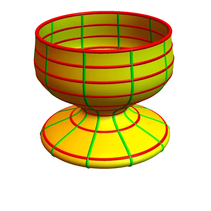
We mostly discuss here the case \(m=2\) and \(n=3\), as we ourselves are made of two-dimensional surfaces, like cells, membranes, skin or tissue. A map \(r: R \subset \mathbb{R}^{2} \rightarrow\) \(\mathbb{R}^{3}\), written as \[r\left(\left[\begin{array}{l}u \\ v\end{array}\right]\right)=\left[\begin{array}{l}x(u, v) \\ y(u, v) \\ z(u, v)\end{array}\right]\] defines a two-dimensional surface. In order to save space, we also just write \(r(u, v)=[x(u, v), y(u, v), z(u, v)]\). In computer graphics, the \(r\) is called \(\boldsymbol{uv}\)-map. The \(u v\)-plane is where you draw a texture. The map \(r\) places it onto the surface. In geography, the map \(r\) is called (surprise!) a map. Several maps define an atlas. The curves \(u \rightarrow r(u, v)\) and \(v \rightarrow r(u, v)\) are called grid curves.
11.2.3 A Look at Parametrization of Spheres and Ellipsoids
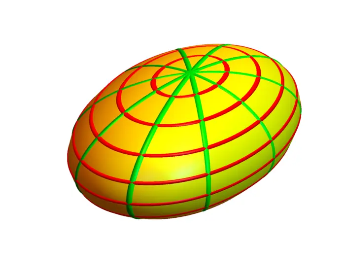
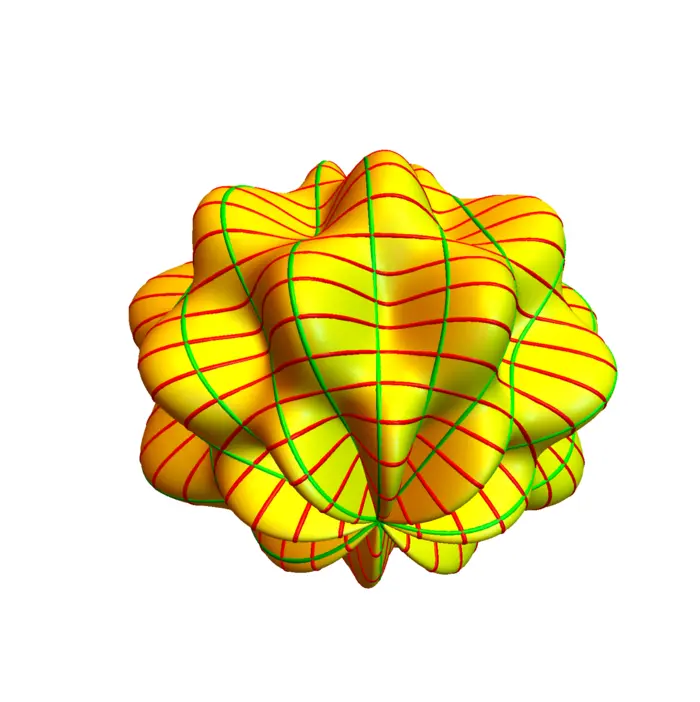
The parametrization \(r(\phi, \theta)=[\sin (\phi) \cos (\theta), \sin (\phi) \sin (\theta), \cos (\phi)]\) produces the sphere \(x^{2}+y^{2}+z^{2}=1\). The full sphere has \(0 \leq \phi \leq \pi\), \(0 \leq \theta<2 \pi\). By modifying the coordinates, we get an ellipsoid \[r(\phi, \theta)=[a \sin (\phi) \cos (\theta), b \sin (\phi) \sin (\theta), c \cos (\phi)]\] satisfying \(x^{2} / a^{2}+y^{2} / b^{2}+z^{2} / c^{2}=1\). By allowing \(a, b, c\) to be functions of \(\phi, \theta\) we get "bumpy spheres" like \[r(\phi, \theta)=\big(3+\cos (3 \phi) \sin (4 \theta)\big)[\sin (\phi) \cos (\theta), \sin (\phi) \sin (\theta), \cos (\phi)].\]
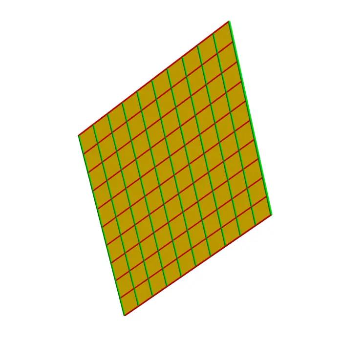
11.2.4 Planes and Grid Curves
Planes are described by linear maps \(r(x)=A x+b\) with \(A \in M(3,2)\) and \(b \in M(3,1)\). The Jacobian map is \(d r=A\). Let \(r_{u}, r_{v}\) be the two column vectors of \(A\). Actually, \(r_{u}\) is a short cut for \(\partial_{u} r(u, v)\), which is the velocity vector of the grid curve \(u \rightarrow r(u, v)\).
11.2.5 Example in Plane Parametrization
An example is the parametrization \(r(u, v)=[u+v-1, u-v+3,3 u-5 v+7]\). In this case \[b=\left[\begin{array}{r}-1 \\ 3 \\ 7\end{array}\right], \quad r_{u}=\left[\begin{array}{l}1 \\ 1 \\ 3\end{array}\right], \quad r_{v}=\left[\begin{array}{r}1 \\ -1 \\ -5\end{array}\right]\] and \[A=d r=\left[\begin{array}{rr}1 & 1 \\ 1 & -1 \\ 3 & -5\end{array}\right].\] We see \[A^{T} A=\left[\begin{array}{lr}11 & -15 \\ -15 & 27\end{array}\right]\] which has determinant \(72\). We also have \[\left|r_{u} \times r_{v}\right|^{2}=\left|\left[\begin{array}{l} 1 \\ 1 \\ 3 \end{array}\right] \times\left[\begin{array}{r} 1 \\ -1 \\ -5 \end{array}\right]\right|^{2}=\left|\left[\begin{array}{r} -2 \\ 8 \\ -2 \end{array}\right]\right|^{2}=72.\]
11.2.6 Unveiling the Distortion Factor: A Connection with the Cross Product
The previous computation suggests a relation between the normal vector and the fundamental form \(g=d r^{T} d r\). In three dimensions, the distortion factor of a parametrization \(r: \mathbb{R}^{2} \rightarrow \mathbb{R}^{3}\) can indeed always be rewritten using the cross product:
Theorem 1. \(\operatorname{det}(d r^{T} d r)=|r_{u} \times r_{v}|^{2}\).
Proof. As \[d r^{T} d r=\left[\begin{array}{ll}r_{u} \cdot r_{u} & r_{u} \cdot r_{v} \\ r_{v} \cdot r_{u} & r_{v} \cdot r_{v}\end{array}\right],\] the identity is the Cauchy-Binet identity \[|r_{u} \times r_{v}|^{2}=|r_{u}|^{2}|r_{v}|^{2}-|r_{u} \cdot r_{v}|^{2}\] which boils down to \(\sin ^{2}(\theta)=1-\cos ^{2}(\theta)\), where \(\theta\) is the angle between \(r_{u}\) and \(r_{v}\). This is the angle between the grid curves you see on the pictures. ◻
11.3 EXAMPLES
Example 1. For the unit sphere \(r(\phi, \theta)=[\sin (\phi) \cos (\theta), \sin (\phi) \sin (\theta), \cos (\phi)]\) and \(A=d r\): \[\begin{aligned} g&=A^{T}A\\ &=\begin{bmatrix} \cos (\phi) \cos (\theta) & \cos (\phi) \sin (\theta) & -\sin (\phi) \\ -\sin (\phi) \sin (\theta) & \sin (\phi) \cos (\theta) & 0 \end{bmatrix} \begin{bmatrix} \cos (\phi) \cos (\theta) & -\sin (\phi) \sin (\theta) \\ \cos (\phi) \sin (\theta) & \sin (\phi) \cos (\theta) \\ -\sin (\phi) & 0 \end{bmatrix} \end{aligned}\] This is \[g=\begin{bmatrix} 1 & 0 \\ 0 & \sin ^{2}(\phi) \end{bmatrix}\] and \(\sqrt{\operatorname{det}(g)}=\sin (\phi)\) is the distortion factor.
Example 2. An important class of surfaces are graphs \(z=f(x, y)\). Its most natural parametrization is \(r(x, y)=[x, y, f(x, y)]\), where the map \(r\) just lifts up the bottom part to the elevated version. An example is the elliptic paraboloid \(r(x, y)=\left[x, y, x^{2}+y^{2}\right]\) and the hyperbolic paraboloid \(r(x, y)=\left[x, y, x^{2}-y^{2}\right]\). We could of course have written also \(r(u, v)=\left[u, v, u^{2}-v^{2}\right]\).
Example 3. A surface of revolution is parametrized like \[r(\theta, z)=[g(z) \cos (\theta), g(z) \sin (\theta), z].\] Note that we can use any variables. In this case, \(u=\theta\), \(v=z\) are used. An example is the cone \(r(\theta, z)=[z \cos (\theta), z \sin (\theta), z]\) or the one-sheeted hyperboloid \[r(\theta, z)=\big[\sqrt{z^{2}+1} \cos (\theta), \sqrt{z^{2}+1} \sin (\theta), z\big].\]
Example 4. The torus is in cylindrical coordinates given as \((r-3)^{2}+z^{2}=1\). We can parametrize this using the polar angle \(\theta\) and the polar angle centered at center of the circle as \[r(\theta, \phi)=\big[\big(3+\cos (\phi)\big) \cos (\theta),\big(3+\cos (\phi)\big) \sin (\theta), \sin (\phi)\big].\] Both angles \(\theta\) and \(\phi\) go from \(0\) to \(2 \pi\). We see now also the relation with the toral coordinates.
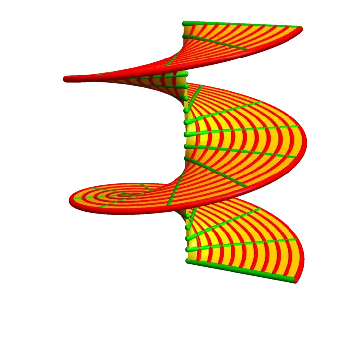
Example 5. The helicoid is the surface you see as a staircase or screw. The parametrization is \(r(\theta, p)=[p \cos (\theta), p \sin (\theta), \theta]\). How can we understand this? The key is to look at grid curves. If \(p=1\), we get a curve \(r(\theta)=[\cos (\theta), \sin (\theta), \theta]\) which we had identified as a helix. On the other hand, if you fix \(\theta\), then you get lines.
11.3.1 Side Remark: Metric Tensors and Riemannian Geometry
The first fundamental form \(g=d r^{T} d r\) is also called a metric tensor. In Riemannian geometry one looks at a manifold \(M\) equipped with a metric \(g\). The simplest case is when \(g\) comes from a parametrization, as we did here. In physics, we know that it is mass which deforms space-time. The quantity \(\|g\|^{2}=\operatorname{det}(g)\) is a multiplicative analogue of \(|g|^{2}=\operatorname{tr}(g)\). For an invertible positive definite square matrix \(A\), we will later see the identity \(\log \operatorname{det}(A)=\operatorname{tr} \log (A)\) which illustrates how both determinant and trace are pivotal numerical quantities derived from a matrix. Trace is additive because of \(\operatorname{tr}(A+B)=\operatorname{tr}(A)+\operatorname{tr}(B)\) and determinant is multiplicative \(\operatorname{det}(A B)=\operatorname{det}(A) \operatorname{det}(B)\) as we will see later.
11.3.2 Ways to Represent a Manifold
To summarize, we have seen so far that there are two fundamentally different ways to describe a manifold. The first is to write it as a level surface \(f=c\) which is a kernel of a map \(g(x)=f-c\). A second is to write it as the image of some map \(r\).
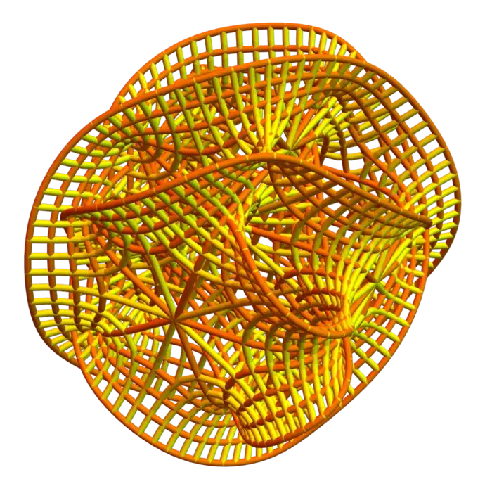
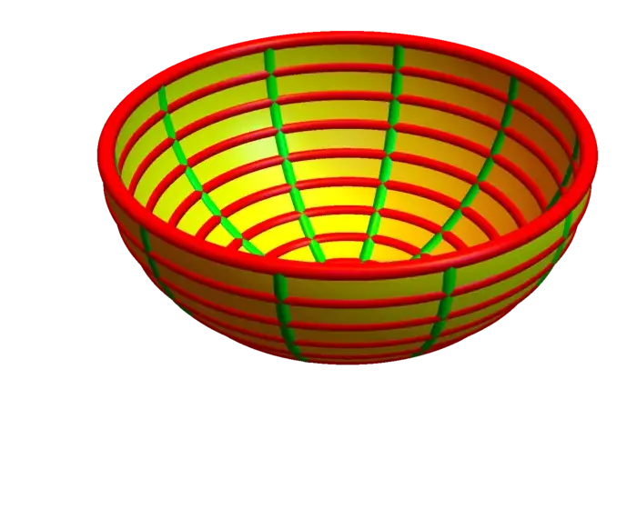
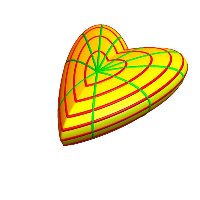
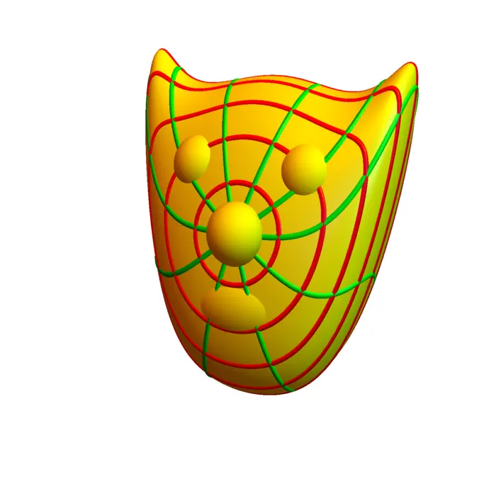
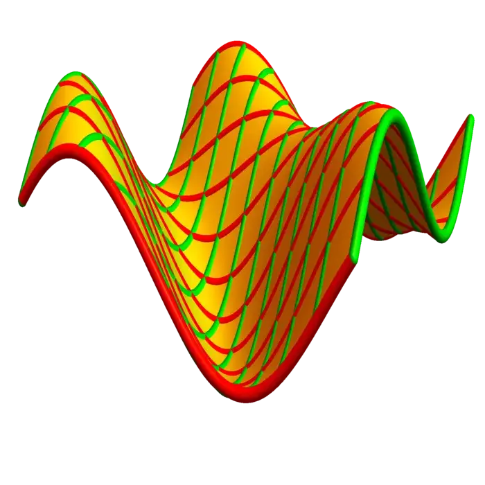
11.4 ILLUSTRATION


EXERCISES
Exercise 1. Parametrize the upper part of the two sheeted hyperboloid \(x^{2}+y^{2}-z^{2}=-1\), \(z>0\) as a surface of revolution.
Exercise 2.
- Parametrize the plane \(x+2 y+3 z-6=0\) using a map \(r: \mathbb{R}^{2} \rightarrow \mathbb{R}^{3}\).
- Now find the matrix \(A=d r\) and compute \(g=A^{T} A\) as well as the distortion factor \(\sqrt{\operatorname{det}(A^{T} A)}\).
- Also compute \(r_{u}\), \(r_{v}\) and \(r_{u} \times r_{v}\) and then compute \(|r_{u} \times r_{v}|\). You should get the same number.
Exercise 3. Given a parametrization \[r(\theta, \phi)=\big[\big(7+2 \cos (\phi)\big) \cos (\theta), \big(7+2 \cos (\phi)\big) \sin (\theta), 2 \sin (\phi)\big]\] of the \(2\)-torus, find the implicit equation \(g(x, y, z)=0\) which describes this torus.
Exercise 4. Parametrize the hyperbolic paraboloid \(z=x^{2}-y^{2}\). What is the first fundamental form \(g=d r^{T} d r\) which is \[\begin{aligned} g = \begin{bmatrix} r_{x} \cdot r_{x} & r_{x} \cdot r_{y} \\ r_{y} \cdot r_{x} & r_{y} \cdot r_{y} \end{bmatrix}? \end{aligned}\] What is the distortion factor \(\sqrt{\operatorname{det}(g)}\)?
Exercise 5. The matrix \(g=d r^{T} d r\) is also called the first fundamental form. If \(r: \mathbb{R}^{4} \to \mathbb{R}^{4}\) is a parametrization of space time then \(g\) is the space time metric tensor. The matrix entries of \(g\) appear in general relativity. Now for some reasons, physics folks use Greek symbols to access matrix entries. They write \(g_{\mu \nu}\) for the entry at row \(\mu\) and column \(\nu\). This appears for example in the Einstein field equations \[R_{\mu \nu}-\frac{1}{2} R g_{\mu \nu}=\frac{8 \pi G}{c^{4}} T_{\mu \nu}.\] We just want you to look up the equation and tell from each of the variables, what it is called and whether it is a matrix, a scalar function or a constant.
- Distinguish \(\|A\|^{2}=\operatorname{det}(A^{T} A)\) and \(|A|^{2}=\operatorname{tr}(A^{T} A)\) in \(M(n, m)\). They only agree for \(m=1\).↩︎