Green's Theorem
Table of Contents
31.1 INTRODUCTION
31.1.1 Electromagnetic Foundations
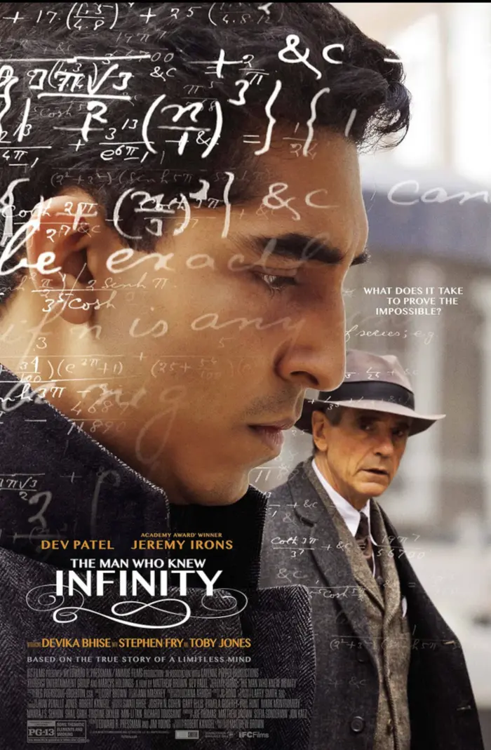
You might have seen the movie "Good Will Hunting" or the movie "The man who knew infinity". The former movie was inspired by Ramanujan, the main character in the second. Unlike "Good Will Hunting", which is pure fiction, the story of Ramanujan is real. He was a self-taught mathematician who made amazing discoveries. There is an older story, which also is true. George Green (1893-1841) was a British mathematician who first described a mathematical framework for electricity and magnetism paving the way for Clerk Maxwell and Lord Kelvin.
31.1.2 Green’s 2D Theorem
The theorem we are going to look at is a theorem about vector fields \(F=[P, Q]\) in the plane. Its derivative \(d F\) is called the curl of \(F\) which is the scalar field \(Q_{x}-P_{y}\). The theorem tells that \[\iint_{G} \,d F \,d A=\int_{\delta G} F \cdot d r\] This is completely analog to \(\int_{I} f^{\prime}(x) \,d x=f(b)-f(a)\) because the later is the integral of \(f\) along the boundary \(\delta G\) of \(I=[a, b]\).

31.1.3 Green’s Unifying Theorem
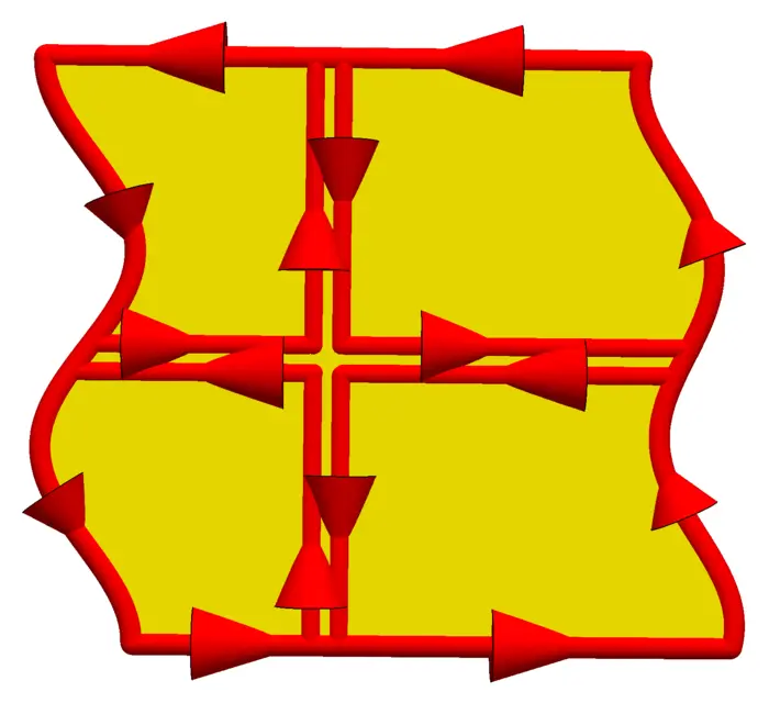
Green’s theorem has been first described by Cauchy. Since Green discovered Gauss Theorem first, the nomenclature of the theorem is a bit strange. Still, since Green saw the general structure of the integral theorems first: integrating the derivative of a field over a manifold is the same than integrating the field over the boundary. In short \(\int_{G} \,d F=\int_{\delta G} F\). When looking at two dimensional objects the derivative of a field \(F=[P, Q]^{T}\) is \(Q_{x}-P_{y}\). The boundary of a planar region is the rim, the curve bounding the region. It is important that the orientation of the curve matches the orientation of the region. We transverse the curve in such a way that the region is to our left.
31.1.4 Notation for Vector Fields and Differential Forms
A remark about notation: we will often also write just \(F\) as a row vector field \(F=[P, Q]\). This is also called a differential \(\boldsymbol{1}\)-form. It is technically correct to write the matrix product \(F \,d r\) instead of the dot product \(F^{T} \cdot d r\). Also, remember that \(d f\) is a row vector field and \(\nabla f=d f^{T}\) a column vector field. Also about notation we should note that it is custom to call continuous functions or fields or curves \(C^{0}\) and functions, fields or curves which are continuously differentiable \(C^{1}\). We most of the time assume in calculus that all objects are at least piecewise \(C^{1}\). Regions can be squares for example but not a region bound by a Koch snowflake.
31.2 LECTURE
31.2.1 Green’s Theorem for Curl and Line Integrals
For a \(C^{1}\) vector field \(F=[P, Q]\) in a region \(G \subset \mathbb{R}^{2}\), the curl is defined as \(\operatorname{curl}(F)=Q_{x}-P_{y}\). Assume the boundary \(C\) of \(G\) oriented so that the region \(G\) is to the left (meaning that if \(r(t)=[x(t), y(t)]\) is a parametrization, then the turned velocity \([-y^{\prime}(t), x^{\prime}(t)]\) cuts through \(G\) close to \(r(t)\)). Green’s theorem assures that if \(C\) is made of a finite collection of smooth curves, then
Theorem 1. \(\iint_{G} \operatorname{curl}(F) \,d x \,d y=\int_{C} F(r(t)) \cdot d r(t)\).
Proof. It is enough to prove the theorem for \(F=[0, Q]\) or \(F=[P, 0]\) separately and for regions \(G\) which are both "bottom to top" \[G=B=\{a \leq x \leq b,\ c(x) \leq y \leq d(x)\}\] and "left to right" \[G=L=\{c \leq y \leq d,\ a(y) \leq x \leq b(y)\}.\] For \(F=[P, 0]\), use a bottom to top integral, where the two vertical integrals along \(r(t)=[b, t]\) and \(r(t)=[a, t]\) are zero. The integrals along \(r(t)=[t, c(t)]\) and \(r(t)=[t, d(t)]\) give \[\begin{aligned} \int_{b}^{b} P(s, c(s)) \,d s-\int_{a}^{b} P(s, d(s)) \,d s&=\int_{a}^{b} \int_{c(t)}^{d(t)}-P_{y}(t, s) \,d s \,d t&\\ &=\iint_{G}-P_{y} \,d s \,d t. \end{aligned}\] For \(F=[Q, 0]\), use a left to right integral, where the bottom and top integrals are zero and where \[\begin{aligned} \int_{c}^{d} Q(b(t), t) \,d t-\int_{c}^{d} Q(a(t), t) \,d t&=\int_{c}^{d} \int_{a(s)}^{b(s)} Q_{x}(t, s) \,d t \,d s\\ &=\iint_{G} Q_{x} \,d s \,d t \end{aligned}\] Together, write \(F=[0, Q]+[P, 0]\), use the first computation for \([P, 0]\) and the second computation for \([0, Q]\). In general, cut \(G\) along a small grid so that each part is of both types. When adding the line integrals, only the boundary survives. ◻


31.2.2 Grid Method
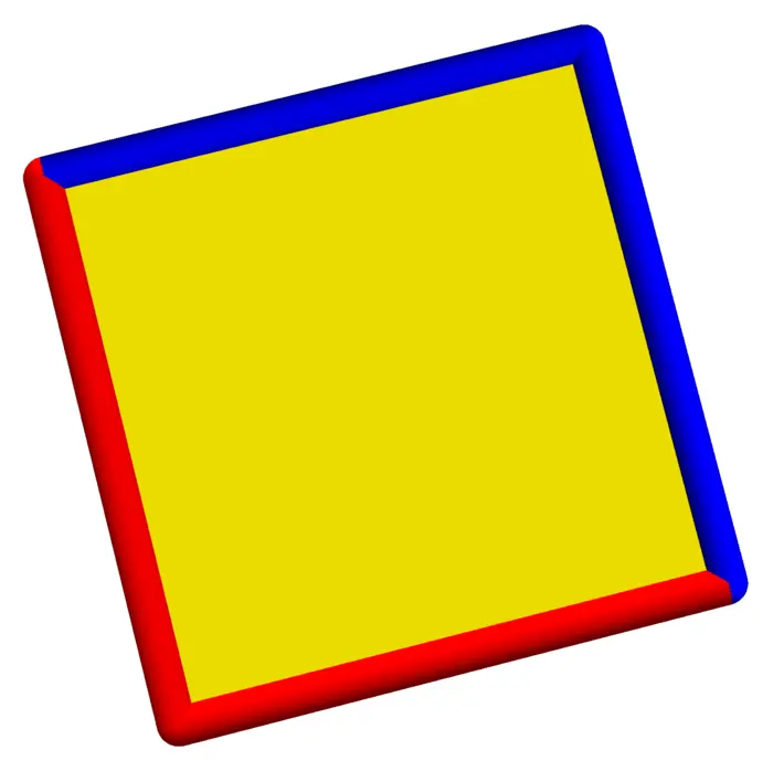
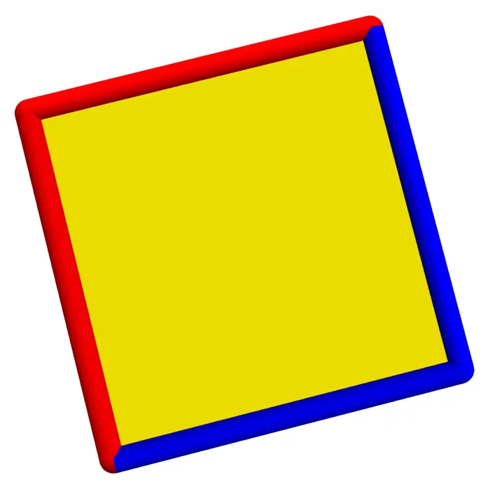
To see that we can cut \(G\) into regions of both types, turn the coordinate system first a tiny bit so that no horizontal nor vertical line segments appear at the boundary. This is possible because we assume the boundary to consist of finitely many smooth pieces. Now also use a slightly turned grid to chop up the region into smaller parts. Now we have a situation where each piece has the form \[G=\{(x, y) \mid c(x) \leq y \leq d(x)\}=\{(x, y) \mid a(y) \leq x \leq b(y)\},\] where \(a\), \(b\), \(c\), \(d\) are piecewise smooth functions.
31.2.3 Conservative Fields in 2D
Green assures:
Theorem 2. If \(F\) is irrotational in \(\mathbb{R}^{2}\), then \(F\) is a gradient field.
31.2.4 Path vs. Curl: Equivalence in 2D
There are four properties which are equivalent if \(F\) is differentiable in \(\mathbb{R}^{2}\):
- \(F\) is a gradient field,
- \(F\) has the closed loop property,
- \(F\) has the path independence property, and
- \(F\) is irrotational.
We have seen in the proof seminar that the vortex vector field \(F=[-y, x] /(x^{2}+y^{2})\) is a counter example to a more general theorem if the field is not differentiable at some point.
31.3 APPLICATIONS
31.3.1 Green’s Theorem for Area Calculation
Green’s theorem allows to compute areas. If \(\operatorname{curl}(F)=1\) and \(C\) is a curve enclosing a region \(G\), then \[\operatorname{Area}(G)=\int_{C} F(r(t)) \cdot r^{\prime}(t) \,d t.\] For example, with \(F=[-y, x] / 2\), and \(r(t)=[a \cos (t), b \sin (t)]\), then \[\begin{aligned} \int_{C} F \cdot d r&=\int_{0}^{2 \pi}\left[\begin{array}{c} -b \sin (t) \\ a \cos (t) \end{array}\right] \cdot\left[\begin{array}{c} -a \sin (t) \\ b \cos (t) / 2 \end{array}\right] dt\\ &=\int_{0}^{2 \pi} a b / 2 \,d t\\ &=\pi a b \end{aligned}\] is the area of the ellipse \(x^{2} / a^{2}+y^{2} / b^{2}=1\).
31.3.2 Area Enclosed by r(t) using Green’s Theorem
What is the area of the region enclosed by \[r(t)=[\cos (t), \sin (t)+\cos (22 t) / 22]?\] Take \(F(x, y)=[0, x]\). The line integral is \[\int_{0}^{2 \pi}[0, \cos (t)] \cdot[-\sin (t), \cos (t)-\sin (22 t)] \,d t=\pi.\]
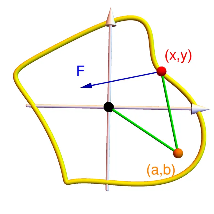
31.3.3 The Planimeter: Green’s Theorem in Action
The planimeter is an analogue computer which computes the area of regions. It works because of Green’s theorem. The vector \(F(x, y)\) is a unit vector perpendicular to the second leg \((a, b) \rightarrow (x, y)\) if \((0,0) \rightarrow (a, b)\) is the second leg. Given \((x, y)\) we find \((a, b)\) by intersecting two circles. The magic is that the curl of \(F\) is constant \(1\). The following computer assisted computation proves this:

31.4 EXAMPLES
Example 1. Problem: Compute \[F(x, y)=[x^{2}-4 y^{3} / 3,8 x y^{2}+y^{5}]\] along the boundary of the rectangle \([0,1] \times[0,2]\) oriented counter clockwise.
Solution: Since \[\operatorname{curl}(F)=Q_{x}-P_{y}=8 y^{2}+4 y^{2}=12 y^{2}\] we have \[\int_{C} F \cdot d r=\int_{0}^{1} \int_{0}^{2} 12 y^{2} \,d y \,d x=32.\]
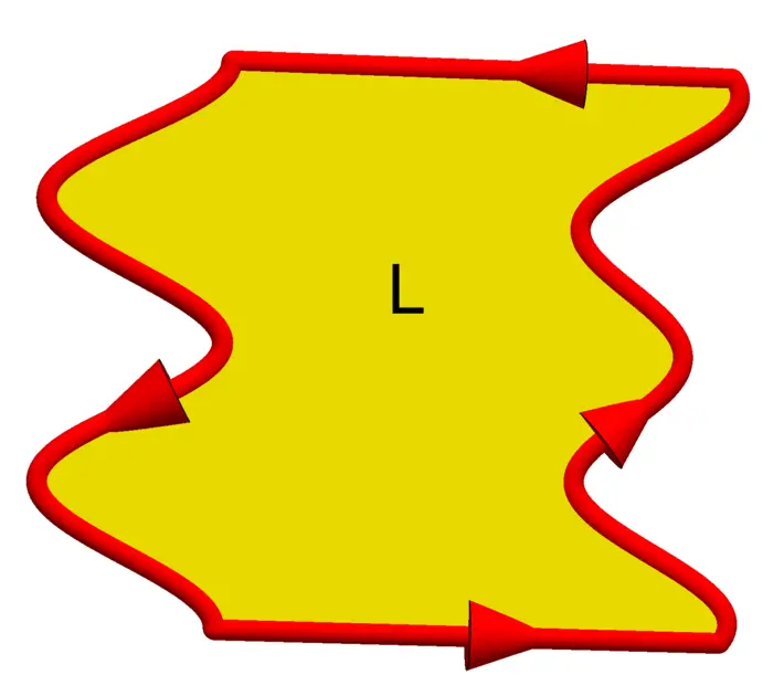
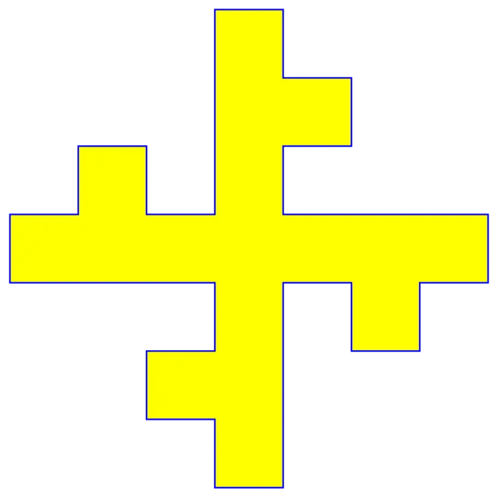
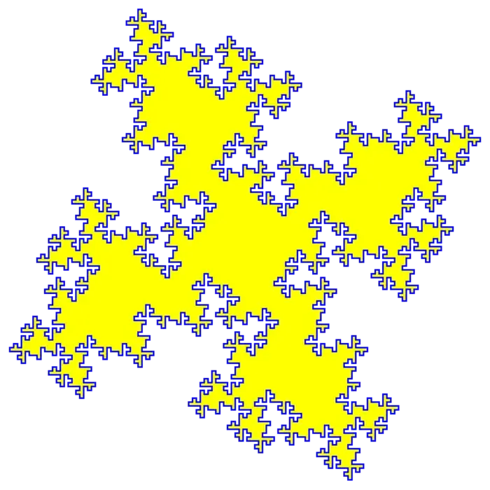
Example 2. Problem: Find the line integral of the vector field \[F(x, y)=\left[\begin{array}{c} x+y \\ 3 x+3 y^{2} \end{array}\right]\] along the boundary \(C\) of the quadratic Koch island. The counter clockwise oriented \(C\) encloses the island \(G\) which has \(289\) unit squares.
Solution: \(\operatorname{curl}(F)=2\), so that \[\iint_{G} 2 \,d A=2 \operatorname{Area}(G)=578.\]

EXERCISES
Exercise 1. Calculate the line integral \(\int_{C} F \cdot d r\) with \[F=[-11 y+3 x^{2} \sin (y)+e^{7777 \sin (x^{6})}, 11 x+x^{3} \cos (y)+2 y e^{22 \sin (y)}]^{T}\] along a triangle \(C\) which traverses the vertices \((0,0)\), \((7,0)\) and \((7,11)\) back to \((0,0)\) in this order.
Exercise 2. A classical problem asks to compute the area of the region bounded by the hypocycloid \[r(t)=[4 \cos ^{3}(t), 4 \sin ^{3}(t)], \quad 0 \leq t \leq 2 \pi.\] We can not do that directly so easily. Guess which theorem to use, then use it!
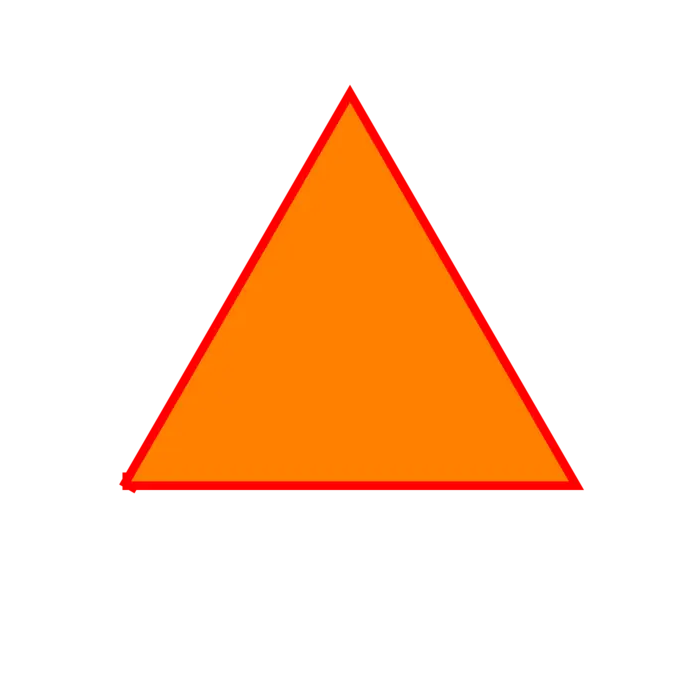
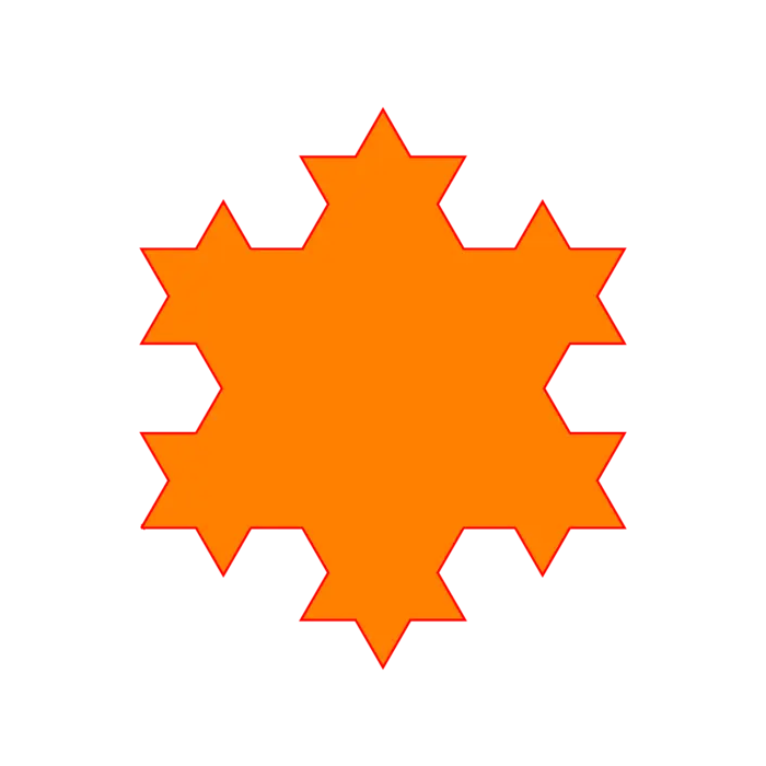
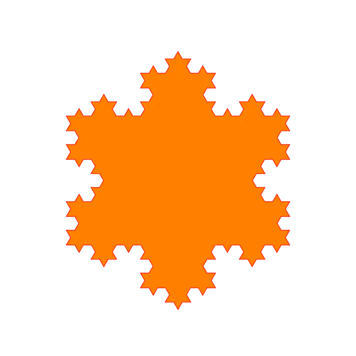
Exercise 3. Find \[\int_{C}[\sin (\sqrt{1+x^{3}}), 7 x] \cdot d r,\] where \(C\) is the boundary of the region \(K(n)\). You see in the picture \(K(0)\), \(K(1)\), \(K(2)\), \(K(3)\), \(K(4)\). The first \(K(0)\) is an equilateral triangle of length \(1\). The second \(K(1)\) is \(K(0)\) with \(3\) equilateral triangles of length \(1 / 3\) added. \(K(2)\) is \(K(1)\) with \(3 \times 4^{1}\) equilateral triangles of length \(1 / 9\) added. \(K(3)\) is \(K(2)\) with \(3 \times 4^{2}\) of length \(1 / 27\) added and \(K(4)\) is \(K(3)\) with \(3 \times 4^{3}\) triangles of length \(1 / 81\) added. What is the line integral in the Koch Snowflake limit \(K=K(\infty)\)? The curve \(K\) is a fractal of dimension \(\log (4) / \log (3)=1.26\ldots\).

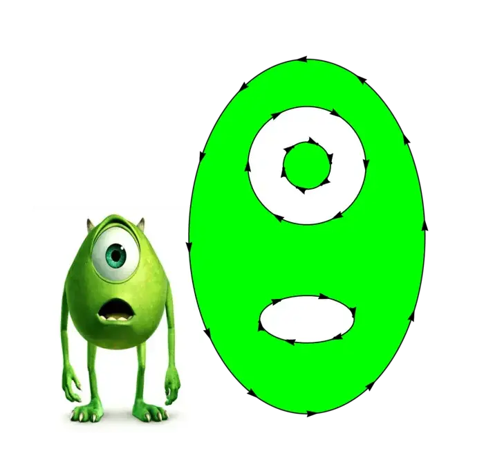
Exercise 4. Given the scalar function \(f(x, y)=x^{5}+x y^{4}\), compute the line integral of \[F(x, y)=[5 y-3 y^{2},-6 x y+y^{4}]+\nabla(f)\] along the boundary of the Monster region given in the picture. There are four boundary curves, oriented as shown in the picture: a large ellipse of area \(16\), two circles of area \(1\) and \(2\) as well as a small ellipse (the mouth) of area \(3\). "Mike" from Monsters, Inc. warns you about orientations!
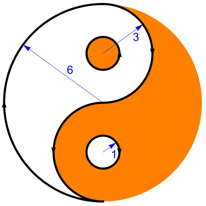
Exercise 5. Let \(C\) be the boundary curve of the white Yang part of the Yin-Yang symbol in the disc of radius \(6\). You can see in the image that the curve \(C\) has three parts, and that the orientation of each part is given. Find the line integral of the vector field \[F(x, y)=[-y+\sin (e^{x}), x]^{T}\] along \(C\). There are three separate line integrals.