Gauss-Jordan Elimination
Table of Contents
2.1 INTRODUCTION
2.1.1 The Evolution of Solving Linear Equation Systems
Systems of linear equations have already been tackled four thousand years ago by Babylonian mathematicians.1 They were able to solve simple systems of equations of two unknown like \(x+y=12\), \(x-y=2\). Chinese mathematicians, in the "Nine chapter of the mathematical art", pushed this to systems of three equations and also to related number theoretical setting appearing in the form of the Chinese remainder theorem. The problem of solving systems of equations appeared also in analysis, like when maximizing functions with constraints. The method of determinants, pioneered by Leibniz, led with Gabriel Cramer to explicit solution formulas of systems or equations. The modern approach of solving systems of equation uses a clear cut elimination process. This process is wicked fast and was formalized by Carl Friedrich Gauss. It is the method we still are using today. It also allows to compute determinants effectively.
2.1.2 Gaussian Elimination
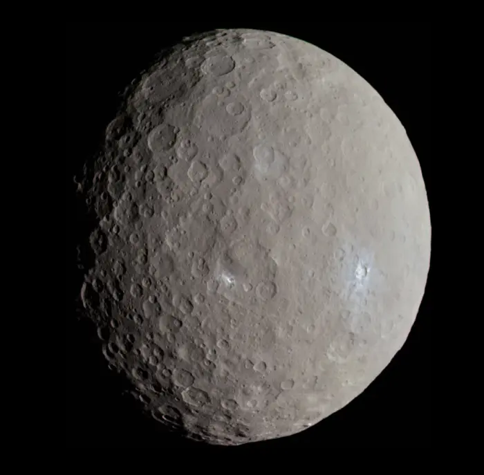
Elimination was of course used long before Gauss. We learn it early on as ordinary elimination. For example, solve for one variable and put it into the rest to have a system with less unknown. What Gauss did was to write down a formal elimination process. This was around 1809. He called the ordinary elimination "eliminationem vulgarem". The process came not out of the blue. The work on rather applied problems must have led to it. For example, Gauss in 1801 was able in a few weeks to predict the path of the minor planet Ceres from \(24\) measurements published in the summer of 1801. It is reported that Gauss needed more than \(100\) hours to determine the \(5\) parameters for the orbit. Exercises like this definitely motivated Gauss for writing down later more formal procedures allowing to solve linear problems or more general data fitting problems. The name "Gaussian elimination" was used first by George Forsythe, while Alan Turing described it in the way we teach it today. We will see here formally that the process determines in a unique way.2
2.2 LECTURE
2.2.1 Linear Transformations and Equations
If an \(n \times m\) matrix \(A\) is multiplied with a vector \(x \in \mathbb{R}^{m}\), we get a new vector \(A x\) in \(\mathbb{R}^{n}\). The process \(x \rightarrow A x\) defines a linear map from \(\mathbb{R}^{m}\) to \(\mathbb{R}^{n}\). Given \(b \in \mathbb{R}^{n}\), one can ask to find \(x\) satisfying the system of linear equations \(A x=b\). Historically, this gateway to linear algebra was walked through much before matrices were even known: there are Babylonian and Chinese roots reaching back thousands of years. 3
2.2.2 Augmented Matrices and Row Reduction
The best way to solve the system is to row reduce the augmented matrix \[B=[A \mid b].\] This is a \(n \times(m+1)\) matrix as there are \(m+1\) columns now. The Gauss-Jordan elimination algorithm produces from a matrix \(B\) a row reduced matrix \(\operatorname{rref}(B)\). The algorithm allows to do three things: subtract a row from another row, scale a row and swap two rows. If we look at the system of equations, all these operations preserve the solution space. We aim to produce leading ones “\(1\)”, which are matrix entries \(1\) which are the first non-zero entry in a row. The goal is to get to a matrix which is in row reduced echelon form. This means:
- every row which is not zero has a leading one,
- every column with a leading \(1\) has no other non-zero entries besides the leading one. The third condition is
- every row above a row with a leading one has a leading one to the left.
2.2.3 Uniqueness of Row Reduced Echelon Form
We will practice the process in class and homework. Here is a theorem
Theorem 1. Every matrix \(A\) has a unique row reduced echelon form.
Proof. 4We use the method of induction with respect to the number \(m\) of columns in the matrix. The induction assumption is the case \(m=1\) where only one column exists. By condition B) there can either be zero or \(1\) entry different from zero. If there is none, we have the zero column. If it is non-zero, it has to be at the top by condition C). We are in row reduced echelon form. Now, let us assume that all \(n \times m\) matrices have a unique row reduced echelon form. Take an \(n \times(m+1)\) matrix \([A \mid b]\). It remains in row reduced echelon form, if the last column \(b\) is deleted (see lemma). Remove the last column and row reduce is the same as row reducing and then delete the last column. So, the columns of \(A\) are uniquely determined after row reduction. Now note that for a row of \([A \mid b]\) without leading one at the end, all entries are zero so that also the last entries agree. Assume we have two row reductions \(\left[A^{\prime} \mid b^{\prime}\right]\) and \(\left[A^{\prime} \mid c^{\prime}\right]\) where \(A^{\prime}\) is the row reduction of \(A\). A leading “\(1\)” in the last column of \(\left[A^{\prime} \mid b^{\prime}\right]\) ) happens if and only if the corresponding row in \(A\) was zero. So, also \(\left[A^{\prime}, c^{\prime}\right]\) has that leading “\(1\)” at the end. Assume now there is no leading one in the last column and \(b_{k}^{\prime} \neq c_{k}^{\prime}\). We have so \(x\), a solution to the equation \(A_{k q}^{\prime} x_{q}+A_{k, q+1}^{\prime} x_{q+1}+\cdots +A_{k, m}^{\prime} x_{m}=b_{k}^{\prime}\). Since solutions to equations stay solutions when row reducing, also \(A_{k q}^{\prime} x_{q}+A_{k, q+1}^{\prime} x_{q+1}+\cdots+A_{k, m}^{\prime} x_{m}=c_{k}^{\prime}\). Therefore \(b_{k}^{\prime}=c_{k}^{\prime}\). ◻
2.2.4 The Lemma of Matrix Partitioning in Proof Construction
A separate lemma allows to break up a proof:
If \([A \mid b]\) is row reduced, then \(A\) is row reduced.
Proof. We have to check the three conditions which define row reduced echelon form. ◻
2.2.5
It is not true that if \(A\) is in row reduced echelon form, then any sub-matrix is in row reduced echelon form. Can you find an example?
2.3 EXAMPLES
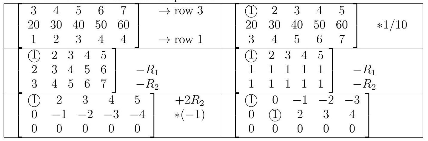
Example 1. To row reduce, we use the three steps and document on the right. To save space, we sometimes report only after having done two steps. We circle the leading \(\boxed{1}\). Note that we did not immediately go to the leading \(\boxed{1}\) by scaling the first. It is a good idea to avoid fractions as much as possible.
Example 2. Finish the following Suduku problem which is a game where one has to fix matrices. The rules are that in each of the four \(2 \times 2\) sub-squares, in each of the four rows and each of the four columns, the entries \(1\) to \(4\) have to appear and so add up to \(10\). \[\begin{bmatrix}2 & 1 & x & 3 \\ 3 & y & z & 1 \\ 4 & 3 & a & 2 \\ b & c & d & e\end{bmatrix}\] We have the equations \[\left\{\begin{aligned} &2+1+x+3=10,\\ &3+y+z+1=10,\\ &4+3+a+2=10,\\ &b+c+d+e=10, \end{aligned}\right.\] for the rows, \[\left\{\begin{aligned} &2+3+4+b=10,\\ &1+y+3+c=10,\\ & x+z+a+d=10,\\ &3+1+2+e+10 \end{aligned} \right.\] for the columns and \[\left\{ \begin{aligned} &2+1+3+y=10,\\ &x+3+z+1=10,\\ &4+3+b+c=10,\\ & a+2+d+e=10 \end{aligned}\right.\] for the four squares. We could solve the system by writing down the corresponding augmented matrix and then do row reduction. The solution is \[\left[\begin{array}{cccc}2 & 1 & 4 & 3 \\ 3 & 4 & 2 & 1 \\ 4 & 3 & 1 & 2 \\ 1 & 2 & 3 & 4\end{array}\right].\]
2.4 ILLUSTRATIONS
The system of equations
$
\left\{\begin{aligned}
&x\phantom{+y+z}+u\phantom{+v+w}&=3\\
&\phantom{x+}y\phantom{+z+u}+v\phantom{+w}&=5\\
&\phantom{x+y+~}z\phantom{+u+v}+w&=9\\
&x+y+z\phantom{+u+v+w}&=8\\
&\phantom{x+y+z+}u+v+w&=9
\end{aligned}
\right.
$
is a tomography problem. These problems appear in magnetic resonance imaging. A precursor was X-ray Computed Tomography (CT) for which Allen MacLeod Cormack got the Nobel in 1979 (Cormack had a sabbatical at Harvard in 1956-1957, where the idea hatched). Cormack lived until 1998 in Winchester MA. He originally had been a physicist. His work had tremendous impact on medicine.
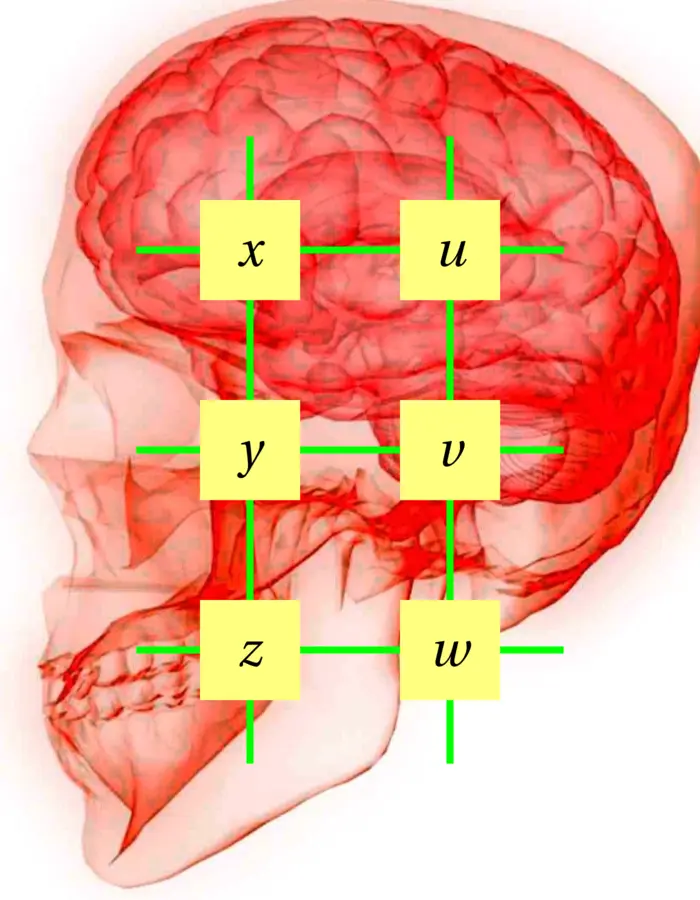
We build the augmented matrix \([A \mid b]\) and row reduce. First remove the sum of the first three rows from the \(4\)’th, then change the sign of the \(4\)’th column: \[\begin{aligned} \left[\begin{array}{ccccccc} \boxed{1} & 0 & 0 & 1 & 0 & 0 & 3 \\ 0 & \boxed{1} & 0 & 0 & 1 & 0 & 5 \\ 0 & 0 & 1 & 0 & 0 & 1 & 9 \\ 1 & 1 & 1 & 0 & 0 & 1 & 8 \\ 0 & 0 & 0 & 1 & 1 & 1 & 9 \end{array}\right] &\Rightarrow\left[\begin{array}{ccccccc} \boxed{1} & 0 & 0 & 1 & 0 & 0 & 3 \\ 0 & \boxed{1} & 0 & 0 & 1 & 0 & 5 \\ 0 & 0 & \boxed{1} & 0 & 0 & 1 & 9 \\ 0 & 0 & 0 & \boxed{1} & 1 & 1 & 9 \\ 0 & 0 & 0 & 1 & 1 & 1 & 9 \end{array}\right]\\ &\Rightarrow\left[\begin{array}{ccccccc} \boxed{1} & 0 & 0 & 0 & -1 & -1 & -6 \\ 0 & \boxed{1} & 0 & 0 & 1 & 0 & 5 \\ 0 & 0 & \boxed{1} & 0 & 0 & 1 & 9 \\ 0 & 0 & 0 & \boxed{1} & 1 & 1 & 9 \\ 0 & 0 & 0 & 0 & 0 & 0 & 0 \end{array}\right] \end{aligned}\]
Now we can read of the solutions. We see that \({v}\) and \({w}\) can be chosen freely. They are free variables. We write \(v=r\) and \(w=s\). Then just solve for the variables:
\[\begin{aligned} x & =-6+r+s \\ y & =5-r \\ z & =9-s \\ u & =9-r-s \\ v & =r \\ w & =s \end{aligned}\]
EXERCISES
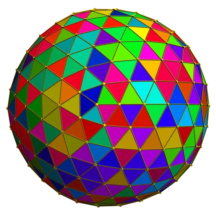
Exercise 1. For a polyhedron with \(v\) vertices, \(e\) edges and \(f\) triangular faces Euler proved his famous formula \(V-E+F=2\). An other relation \(3 F=2 E\) called a Dehn-Sommerville relation holds because each face meets \(3\) edges and each edge meets \(2\) faces. Assume the number \(F\) of triangles is \(F=540\). Write down a system of equations for the unknowns \(V, E, F\) in matrix form \(A x=b\), then solve it using Gaussian elimination.
Exercise 2. Row reduce the matrix \(A=\begin{bmatrix}1 & 2 & 3 & 4 & 5 \\ 1 & 2 & 3 & 4 & 0 \\ 1 & 2 & 3 & 0 & 0\end{bmatrix}\).
Exercise 3. In the "Nine Chapters on Arithmetic", the following system of equations appeared \[\begin{aligned} & 3 x+2 y+z=39 \\ & 2 x+3 y+z=34 \\ & x+2 y+3 z=26 \end{aligned}\] Solve it using row reduction by writing down an augmented matrix and row reduce.
Exercise 4.
- Which of the following matrices are in row reduced echelon form? \[\begin{aligned} A= \begin{bmatrix} 1 & 1 & 0 & 1 \\ 0 & 0 & 1 & 0 \end{bmatrix}, \quad B= \begin{bmatrix} 0 & 0 & 1 \\ 0 & 1 & 0 \end{bmatrix}, \quad C= \begin{bmatrix} 0 & 0 & 1 \\ 0 & 0 & 0 \end{bmatrix}, \quad D= \begin{bmatrix} 0 & 0 \\ 0 & 1 \end{bmatrix}. \end{aligned}\]
- Two \(n \times m\) matrices in reduced row-echelon form are called of the same type if they contain the same number of leading \(1\)’s in the same positions. For example, \(\big[\begin{smallmatrix}1 & 2 & 0 \\ 0 & 0 & 1\end{smallmatrix}\big]\) and \(\big[\begin{smallmatrix}1 & 3 & 0 \\ 0 & 0 & 1\end{smallmatrix}\big]\) are of the same type. How many types of \(2 \times 2\) matrices in reduced row-echelon form are there?
Exercise 5. Given \(A=\begin{bmatrix}1 & 2 & 3 \\ 4 & 5 & 6 \\ 7 & 8 & 9\end{bmatrix}\). Compare \(\operatorname{rref}\left(A^{T}\right)\) with \((\operatorname{rref}(A))^{T}\). Is it true that the transpose of a row reduced matrix is a row reduced matrix?
- I checked with Ajak who also hinted, that Phastos might have leaked Gauss-Jordan elimination. The opening scene in the newest Marvel’s movie shows the eternals arriving here 5000 BC.↩︎
- J.F. Grcar, Mathematicians of Gaussian Elimination, Notices of the AMS, 58, 2011.↩︎
- For more, look at the exhibit on the website of the 2018 Math 22a.↩︎
- The proof is well known: i.e. Thomas Yuster, Mathematics Magazine, 1984.↩︎