Extrema
Table of Contents
- 19.1 INTRODUCTION
- 19.2 LECTURE
- 19.2.1 Finding Optima with Gradients
- 19.2.2 Unveiling Critical Points
- 19.2.3 The Second Derivative Test Steps In
- 19.2.4 Positive and Negative Definite Matrices
- 19.2.5 Unveiling the Role of Positive Definite Hessians
- 19.2.6 Classifying Extrema in Two Dimensions
- 19.2.7 Morse Functions and the Second Derivative Test
- 19.2.8 From Hessian to Gauss Curvature
- 19.2.9 The Morse Lemma
- 19.3 EXAMPLES
- EXERCISES
19.1 INTRODUCTION
19.1.1 Exploring Learning as an Optimization Process
Learning is an optimization process with the goal to increase knowledge, skills and creative power. This applies both for education as well as for machine learning. In order to track the learning process, we need a function which measures progress. An old fashioned metric is the GPA averaging some grades in an educational system, an other or IQ scores measured by doing tests. An other metric example in a research setting is a social network score like the number of citations or the h-index. For a car driving autonomously it could be the \(f(x)=100 /(1+N(x))\) where \(N(x)\) is the number of accidents produced using the parameter configuration \(x\) in a fixed period.
19.1.2 Will AI Conquer Every Domain?
Once the frame work and the function \(f\) is fixed, the question is how to increase \(f\) most effectively. This simplistic picture is quite effective both for human intelligence or artificial intelligence. For many functions which have been considered (winning in chess games, computational power, data retention, feature detection, driving cars or flying planes) machines progressed rapidly. There is hardly anybody who seriously doubts that humans eventually will lose the battle for any function \(f\) which can be considered. There are still domains where machines have not taken over. Examples are art or writing scientific papers.1
19.1.3 Machine Learning’s Advantage in Gradient-Based Optimization
Once a machine knows the function \(f\), it can quit comfortably determine from a position \(x\) in which direction to change to increase \(f\) most rapidly. The direction of fastest increase is the direction of the gradient \(\nabla f\) of \(f\). In calculus, we look at situations, where the position consists of a few variables only. Single variable calculus deals with the situation of one variable. We look here at the situation with \(n\) variables but will mostly work with \(2\) variables as this already gives the main idea. The principle is that we have reached an optimum where no change any more can increase the function \(f\). This means mathematically that the derivative \(d f\) of \(f\) is zero. We call such points "critical points".
19.1.4 Using Gradients to Find the Direction of Improvement
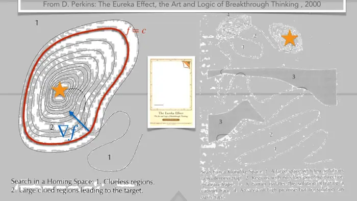
Let us first look at the rate of change of a function along a direction \(v\). Take a curve \(r(t)=x+t v\) where \(v\) is a unit vector. By the chain rule, the rate of change at \(x\) is given by \[f(r(t))=\nabla f(r(t)) \cdot r^{\prime}(0)=\nabla f(x) \cdot v.\] We know for the dot product that this is equal to \[|\nabla f(x)||v| \cos (\alpha)=|\nabla f(x)| \cos (\alpha).\] This is maximized for \(\cos (\alpha)=1\) which means that \(v\) points into the same direction than \(\nabla f\). So, The gradient points into the direction of maximal increase. This is important to remember. If you are in a landscape given by the height \(f(x)\) you have to go into the direction of \(\nabla f(x) /|\nabla f(x)|\) in order to increase most. Of course, this does not make sense if \(\nabla f(x)=0\) but that is the situation where you are at a maximum, and where you can not increase \(f\) any more.
19.2 LECTURE
19.2.1 Finding Optima with Gradients
All functions are assumed here to be in \(C^{2}\), meaning that they are two times continuously differentiable. It all starts with an observation going back to Pierre de Fermat:
Theorem 1. If \(x_{0}\) is a maximum of \(f: \mathbb{R}^{m} \rightarrow \mathbb{R}\), then \(\nabla f(x_{0})=0\).
Proof. We prove this by contradiction. Assume \(\nabla f(x_{0}) \neq 0\), define the vector \(v=\) \(\nabla f(x_{0})\) and look at \(g(t)=f(x_{0}+t v)\), which is a function of one variable. By the chain rule, it satisfies \[g^{\prime}(0)=\nabla f(x_{0}+0 v) \cdot v=|\nabla f|^{2}>0.\] This means that \(f(x_{0}+t v)>0\) for small \(t>0\). The point \(x_{0}\) can not have been maximal. This is a contradiction. ◻
19.2.2 Unveiling Critical Points
A point \(x\) with \(\nabla f(x)=0\) is called a critical point of \(f\). By the Taylor formula, we have at a critical point \(x_{0}\) the quadratic approximation \[Q(x)=f(x_{0})+(x-x_{0})^{T} H(x_{0})(x-x_{0}) / 2,\] where \(H(x_{0})\) is the Hessian matrix \[H(x_{0})=\left[\begin{array}{llll} f_{x_{1} x_{1}} & f_{x_{1} x_{2}} & \cdots & f_{x_{1} x_{m}} \\ f_{x_{2} x_{1}} & f_{x_{2} x_{2}} & \cdots & f_{x_{2} x_{m}} \\ \cdots & \cdots & \cdots & \cdots \\ f_{x_{m} x_{1}} & f_{x_{m} x_{2}} & \cdots & f_{x_{m} x_{m}} \end{array}\right].\]
19.2.3 The Second Derivative Test Steps In
As in one dimension, having a critical point does not assure that a point is a local maximum or minimum. The second derivative test in single variable calculus assures that if \(f^{\prime}(x_{0})=0\), \(f^{\prime \prime}(x_{0})>0\), we have a local minimum and if \(f^{\prime}(x_{0})=0\), \(f^{\prime \prime}(x_{0})<0\), we have a local maximum. If \(f^{\prime \prime}(x_{0})=0\), we can not say anything without looking at higher derivatives.
19.2.4 Positive and Negative Definite Matrices
A matrix \(A\) is called positive definite if \(v \cdot A v>0\) for all vectors \(v \neq 0\). It is called negative definite if \(v \cdot A v<0\) for all vectors \(v \neq 0\). A diagonal matrix with positive diagonal entries is positive definite. In the following statements, we assume \(x_{0}\) is a critical point.
19.2.5 Unveiling the Role of Positive Definite Hessians
We say \(x_{0}\) is a local maximum of \(f\) if there exists \(r>0\) such that \(f(x) \leq f(x_{0})\) for all \(|x-x_{0}|
Theorem 2. Assume \(\nabla f(x_{0})=0\). If \(H(x_{0})\) is positive definite, then \(x_{0}\) is a local minimum. If \(H(x_{0})\) is negative definite, then \(x_{0}\) is a local maximum.
Proof. As \(\nabla f(x_{0})=0\), the quadratic approximation at \(x_{0}\) is \[Q(x)=f(x_{0})+H(x_{0}) v \cdot v / 2>f(x_{0})\] for small non-zero \(v=x-x_{0}\) and Hessian \(H\). The analogue statement for the minimum can be deduced by replacing \(f\) with \(-f\). ◻
19.2.6 Classifying Extrema in Two Dimensions
Let us look at the case, where \(f(x, y)\) is a function of two variables such that \(f_{x}(x_{0}, y_{0})=0\) and \(g_{x}(x_{0}, y_{0})=0\). The Hessian matrix is
\[H(x_{0}, y_{0})=\left[\begin{array}{ll} f_{x x} & f_{x y} \\ f_{y x} & f_{y y} \end{array}\right]\]
In this two dimensional case, we can classify the critical points if the determinant \[D=\operatorname{det}(H)=f_{x x} f_{y y}-f_{x y}^{2}\] of \(H\) is non-zero. The number \(D\) is also called the discriminant at a critical point.

19.2.7 Morse Functions and the Second Derivative Test
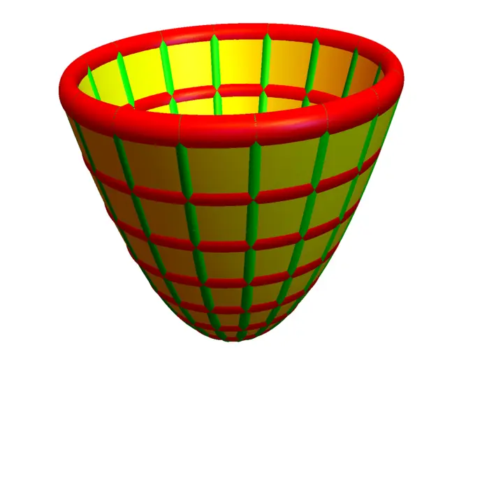
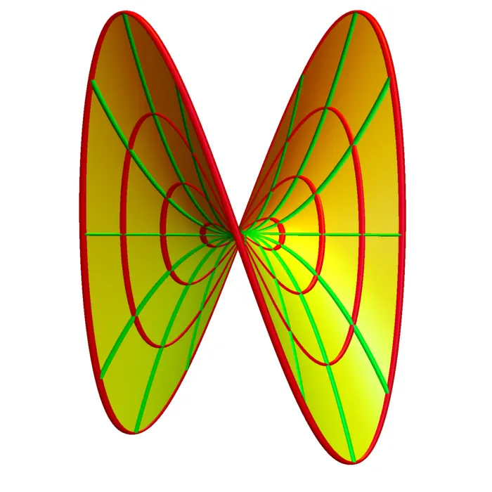
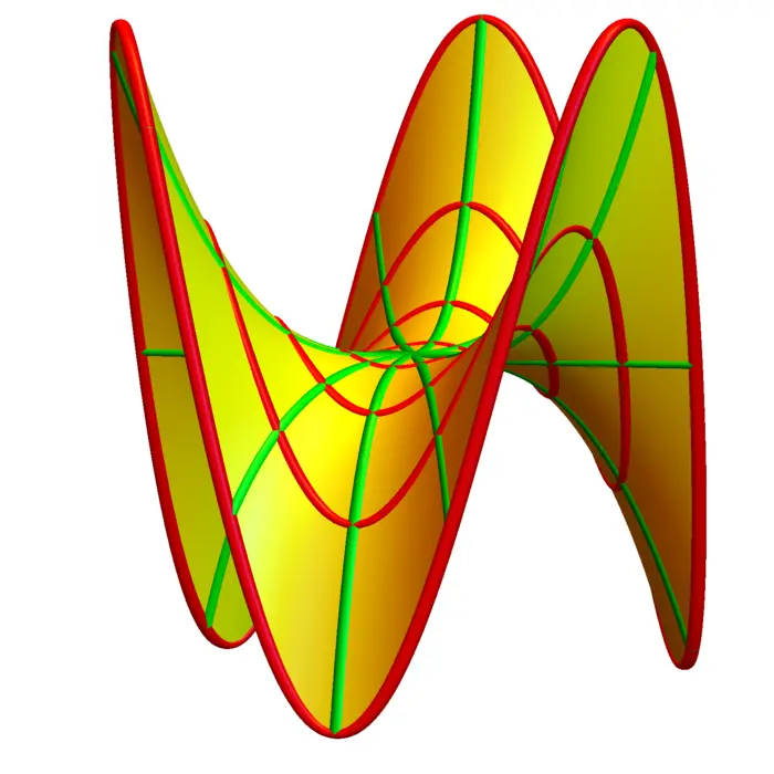
We say \((x_{0}, y_{0})\) is a Morse point, if \((x_{0}, y_{0})\) is a critical point and the determinant is non-zero. A \(C^{2}\) function is a Morse function if every critical point is Morse. Examples of Morse functions are \(f(x, y)=x^{2}+y^{2}\), \(f(x, y)=-x^{2}-y^{2}\) and \(f(x, y)=x^{2}-y^{2}\). The last case is called a hyperbolic saddle. In general, a critical point is a hyperbolic saddle if \(D \neq 0\) and if it is neither a maximum nor a minimum. Here is the second derivative test in dimension \(2\):
Theorem 3. Assume \(f \in C^{2}\) has a critical point \((x_{0}, y_{0})\) with \(D \neq 0\).
- If \(D>0\) and \(f_{x x}>0\) then \((x_{0}, y_{0})\) is a local minimum.
- If \(D>0\) and \(f_{x x}<0\) then \((x_{0}, y_{0})\) is a local maximum.
- If \(D<0\) then \((x_{0}, y_{0})\) is a hyperbolic saddle.
Proof. After translation \((x, y) \rightarrow(x-x_{0}, y-y_{0})\) and replacing \(f\) with \(f-\) \(f(x_{0}, y_{0})\), we have \((x_{0}, y_{0})=(0,0)\) and \(f(0,0)=0\). At the critical point, the quadratic approximation is now \[Q(x, y)=a x^{2}+2 b x y+c y^{2}.\] This can be rewritten as \[a\big(x+\frac{b}{a} y\big)^{2}+\big(c-\frac{b^{2}}{a}\big) y^{2}=a(A^{2}+D B^{2})\] with \[A=\big(x+\frac{b}{a} y\big), \quad B=b^{2} / a^{2}\] and discriminant \(D\). If \(a=f_{x x}>0\) and \(D>0\) then \(c-b^{2} / a>0\) and the function has positive values for all \((x, y) \neq(0,0)\). The point \((0,0)\) is then a minimum. If \(a=f_{x x}<0\) and \(D>0\), then \(c-b^{2} / a<0\) and the function has negative values for all \((x, y) \neq(0,0)\) and the point \((x, y)\) is a local maximum. If \(D<0\), then \(f\) takes both negative and positive values near \((0,0)\). ◻
19.2.8 From Hessian to Gauss Curvature
One can ask, why \(f_{x x}\) and not \(f_{y y}\) is chosen. It does not matter, because if \(D>0\), then both \(f_{x x}\) and \(f_{y y}\) need to be non-zero and have the same sign. Instead of \(f_{x x}\), one could also have pick the more natural trace \(\operatorname{tr}(H)\). It is invariant under coordinate changes similarly as the determinant \(D\). The discriminant \(D\) happens also to be the Gauss curvature of the surface at the point.
19.2.9 The Morse Lemma
In higher dimensions, the situation is described by the Morse lemma. It tells that near a critical point there is a coordinate change \(\phi\) such that \(g(x)=f(\phi(x))\) is a quadratic function \(f(x)=B(x-x_{0}) \cdot(x-x_{0})\) where \(B\) is diagonal with entries \(+1\) or \(-1\). Critical point can then be given a Morse index, the number of entries \(-1\) in \(B\). The Morse lemma is actually a theorem (theorems are more important than lemmata=helper theorems)
Theorem 4. Near a Morse critical point \(x_{0}\) of a \(C^{2}\) function \(f\), there is a coordinate change \(\phi: \mathbb{R}^{m} \rightarrow \mathbb{R}^{m}\) such that \(g(x)=f(\phi(x))-f(x_{0})\) is \[g(x)=-x_{1}^{2}-\cdots-x_{k}^{2}+x_{k+1}^{2}+\cdots+x_{m}^{2}.\]
Proof. We use induction with respect to \(m\).
- Induction foundation: For \(m=1\), the result tells that for a Morse critical point, the function looks like \(y=x^{2}\) or \(y=-x^{2}\). First show that if \(f(0)=f^{\prime}(0)=0\), \(f^{\prime \prime}(0) \neq 0\), then \(f(x)=x^{2} h(x)\) or \(f(x)=-x^{2} h(x)\) for some positive \(C^{2}\) function \(h\). Proof. By a linear coordinate change we assume \(x_{0}=0\) and \(f(0)=0\). There exists then \(g(x)\) such that \(f(x)=x g(x)\): it is \(g(x)=f(x) / x\) for \(x \neq 0\) and is in the limit \(x \rightarrow 0\) the value of \(\lim _{x \rightarrow 0}(f(x)-\) \(f(0)) / x=f^{\prime}(0)\). By the product rule, \(f^{\prime}(x)=g(x)+x g^{\prime}(x)\) with \(g(0)=0\). Because \(f^{\prime}(0)=g(0)=0\) can define \(f(x) / x^{2}\) for \(x \neq 0\) and take the limit \(x \rightarrow 0\), because by applying Hôpital twice, the limit is \(f^{\prime \prime}(0)\). The coordinate change is now given by a function \(y=\phi(x)\) satisfying \(g(x, y)=y \sqrt{h(y)}=x\). Implicit differentiation gives \(g_{y}(0,0)=\sqrt{h(y)} \neq 0\) so that by the implicit function theorem \(y(x)\) exists.
- Induction step \(\boldsymbol{m \rightarrow m+1}\): we first note that Taylor for \(C^{2}\) with remainder term implies that \(f(x_{1}, \ldots, x_{n})=\sum_{i, j} x_{i} x_{j} h_{i j}(x_{1}, \ldots, x_{n})\) with some continuous functions \(h_{i j}\). Furthermore, the function value \(h_{i j}(0)=f_{x_{i} x_{j}}(0)=H_{i j}(0)\) are the coordinates of the Hessian. Apply first a rotation so that \(h_{11} \neq 0\). Now look at \(x_{1}\) and keep the other coordinates constant. As in (i), find a coordinate change \(\phi\) such that \(f(\phi(x))=\pm x_{1}^{2}+g(x_{2}, \ldots, x_{m})\), where \(g\) inherits the properties of but is of one dimension less. By induction assumption, there is a second coordinate change such that \[g(\psi(x))=x_{2}^{2}-\cdots-x_{l}^{2}+x_{l+1}^{2}+\cdots+x_{m}^{2}.\] Combining \(\phi\) and \(\psi\) produces the Morse normal form.
◻
19.3 EXAMPLES
Example 1. Q: Classify the critical points of \(f(x, y)=x^{3}-3 x-y^{3}-3 y\).
A: As \[\nabla f(x, y)=\left[3 x^{2}-3,-3 y^{2}+3\right]^{T},\] the critical points are \((1,1)\), \((-1,1)\), \((1,-1)\) and \((-1,-1)\). We compute \[H(x, y)=\left[\begin{array}{cc}2 x & 0 \\ 0 & -2 y\end{array}\right].\] For \((1,1)\) and \((-1,-1)\) we have \(D=-4\) and so saddle points. For \((-1,1)\), we have \(D=4\), \(f_{x x}=-2\), a local max. For \((1,-1)\) where \(D=4\), \(f_{x x}=2\) we have a local min.
EXERCISES
Exercise 1.
- Classify the critical points of the function \[f(x, y)=x^{2}+y^{3}-x y.\] (Maxima, minima or saddle points).
- Now do the same for \[f(x, y, z)=x^{2}+y^{3}-x y+z^{2}\] and find the Morse index at each critical point.
Exercise 2. Find all critical points of the \(\boldsymbol{3}\)D area \(\boldsymbol{51}\) function \[f(x, y, z)=x^{51}-51 x+y^{51}-51 y+z^{51}-51 z.\] Compute the Hessian \(H=d^{2} f\) at each critical point and determine the maxima (all eigenvalues are negative) and minima (all eigenvalues are positive).
P.S. Area \(51\) is an old hat. But \(3\)D Area \(51\) is still highly classified and rumored to be near the dark side of the moon.
Exercise 3. Where on the parametrized surface \(r(u, v)=[u^{2}, v^{3}, u v]\) is the temperature \(T(x, y, z)=12 x+y-12 z\) minimal. Classify all the critical points of the function \(f(u, v)=T(r(u, v))\). [If you have found the function \(f(u, v)\), you can replace \(u\), \(v\) again with \(x\), \(y\) if you like to work with a function \(f(x, y)\).]
Exercise 4. Find all the critical points of the function \[f(x, y, z)=(x-1)^{2}-y^{2}+x z^{2}.\] In each of the cases, find the Hessian matrix. Also here compute the eigenvalues. These are numbers \(\lambda\) such that \(H v=\lambda v\) for some non-zero vector. One can find them by looking for the roots of the characteristic polynomial \(\chi_{H}(\lambda)=\operatorname{det}(L-\lambda)\). You can calculate them on a computer. Find in each case the eigenvalues.
Exercise 5.
- Find a function \(f(x, y)\) with \(3\) maxima and \(3\) saddle points and one minimum.
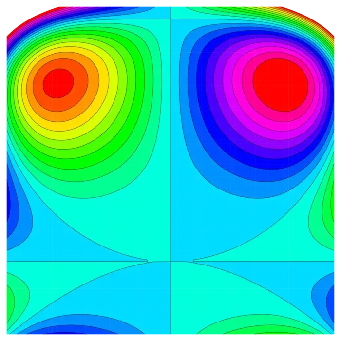
- You see below a contour map of a function of two variables. How many critical points are there? Is the function a Morse function?
- There could be resistance: humans might decide not to cite scientific breakthroughs by machines. On the other hand, who would not want to learn a "theory of everything" even if it is discovered by a machine?↩︎