Double Integrals
Table of Contents
22.1 INTRODUCTION
22.1.1 Beyond 1D: Area and Integrals
When integrating a continuous function \(f(x, y)\) over a two-dimensional domain \(R \subset \mathbb{R}^{2}\), we can use Riemann sums again like in one dimensions and get \(\iint_{R} f(x, y) \,d A\). A special case of a continuous function is the function \(f(x, y)=1\). If we integrate \(\iint_{R} 1 \,d A\) we get the area. Unlike in one dimensions, where a domain is just an interval, we can have much more interesting regions in two dimensions.
22.1.2 Higher Dimensions, More Integrals
Integration in two dimensions is a good prototype. Knowing this multi-dimensional situation, will allow also to understand how to integrate in \(3\) or more dimensions. We will learn next week how to compute the area of a surface. But dimensional integrals also matter in higher dimensions: if we integrate a so called \(2\)-form \(F\) over a two-dimensional surface, we get double integrals. An example of a \(2\)-form is the electromagnetic field also known as "light". String theorists work in higher dimensional spaces. The surface traced out by a moving string is a \(2\)-dimensional surface called a "world-sheet". Its surface area is called the Nambu-Goto action which plays the role of the length in classical mechanics. This is a double integral.
22.1.3 Calculus, Integration, and The Unknown
Like particle move on shortest paths called geodesics, strings move on paths in which the surface area is minimized. Not everybody has jumped onto the string theory wagon however and the theory lead to a dead end. We do not know yet. In any case, in the quest of understanding the basic building blocks of space and time and matter is exciting. We live in an interesting time where highly successive theories like the standard model (SM), quantum mechanics (QM) or general relativity (GR) match measurements with enormous precision. There are also other interesting theories which lack experimental verifications. Without doubt however, calculus and integration theory in particular will play an important role also in the future, whatever lies ahead.
22.2 LECTURE
22.2.1 Double Integral and Its Existence
Given a bounded region \(R\) in \(\mathbb{R}^{2}\) and a continuous function \(f(x, y): R \rightarrow \mathbb{R}\), define the Riemann integral \(I=\iint_{R} f(x, y) \,d A\) as the \(n \rightarrow \infty\) limit of \[I_{n}=\sum_{(\frac{i}{n}, \frac{j}{n}) \in R} f\Big(\frac{i}{n}, \frac{j}{n}\Big) \,\frac{1}{n^{2}}.\] The bounded region \(R\) is a defined as closed subset of \(\mathbb{R}^{2}\) bound by finitely many differentiable curves \(R=\left\{g_{1} \leq c_{1}, \ldots, g_{k} \leq c_{k}\right\}\). As already in one dimension, the definition is designed to be independent of an orientation chosen on \(R\). We are integrating like summing up a spread sheet. Just add up all entries. To justify that the limit exists, we again can use the Heine-Cantor theorem which tells that \(f\) is continuous on \(R\) if and only if it is uniformly continuous. This means there are numbers \(M_{n} \rightarrow 0\) such that if \(|(x_{1}, y_{1})-(x_{2}, y_{2})| \leq 1 / n\), then \(|f(x_{1}, y_{1})-f(x_{2}, y_{2})| \leq M_{n}\).
Theorem 1. For continuous \(f\) on a bounded region \(R, \iint_{R} f \,d x \,d y\) exists.
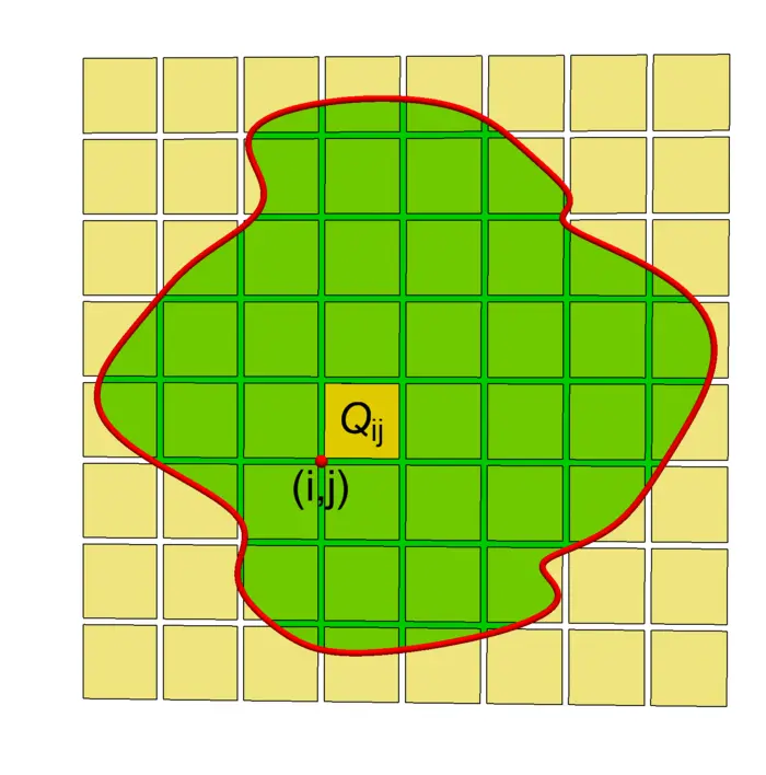
Proof. In each cube \[Q_{i j}=\{i / n \leq x \leq(i+1) / n,\ j / n \leq y \leq(j+1) / n\} \cap R\] define \(a_{i j}=\min _{(x, y) \in Q_{i j}} f(x, y)\) and \(b_{i j}=\max _{(x, y) \in Q_{i j}} f(x, y)\). Because the boundary was assumed to be given by a collection of curves which have finite total arc length \(L\), the number of cubes \(Q_{i j}\) which intersect the boundary \(C\) is bounded by \(4 L n\) (a curve of length 1 can maximally touch 4 squares). Define also \(F=\max _{(x, y) \in R}|f(x, y)|\). We have with \(K_{n}=4 L F / n\): \[A_{n}-K_{n} \leq I_{n} \leq B_{n}+K_{n}\] where \(A_{n}=\sum_{i, j} a_{i j} / n^{2}\) and \(B_{n}=\sum_{i, j} b_{i j} / n^{2}\) and \(K_{n}\) takes care of cubes \(Q_{i j}\) which intersect the boundary of \(R\) and so only contribute partially. Let \(I\) be the limsup of \(I_{n}\). We have \[B_{n}-A_{n} \leq M_{n} n^{2} / n^{2}=M_{n} \rightarrow 0\] and \(K_{n} \rightarrow 0\) as well so that \(|I_{n}-I| \leq M_{n}+K_{n} \rightarrow 0\). ◻
22.2.2 Fubini’s Theorem
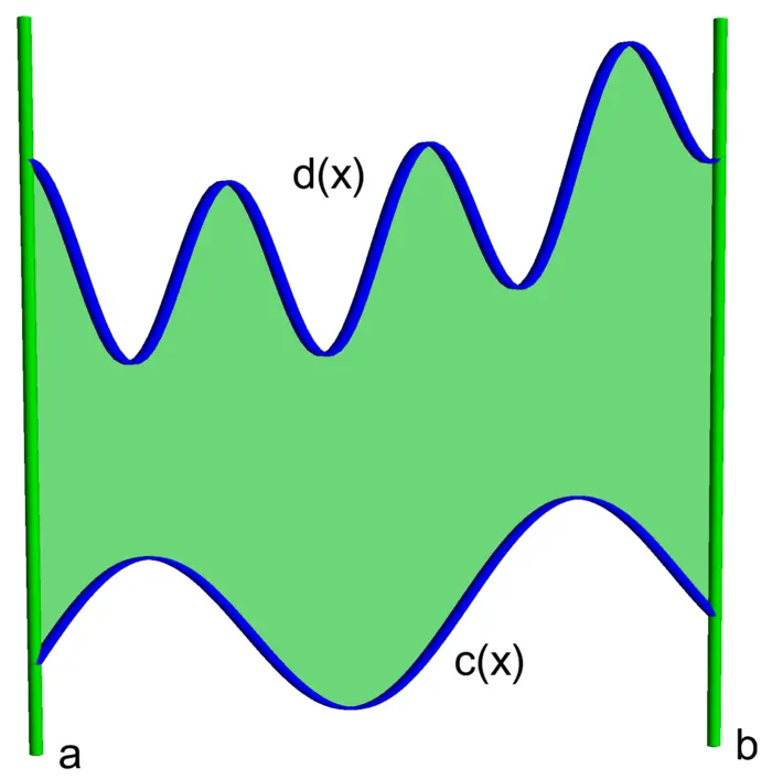
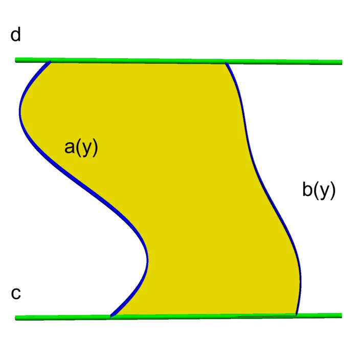
We rarely evaluate integrals using Riemann sums. Fortunately it is possible to reduce a double integral to single integrals. One can do that for basic regions which consist of two type of regions "bottom to top" regions \[R=\{(x, y) \mid a \leq x \leq b,\ c(x) \leq y \leq d(x)\}\] or "left to right" regions \[R=\{(x, y) \mid a(y) \leq x \leq b(y),\ c \leq y \leq d\}.\] By cutting a general region into smaller pieces like intersecting with sufficiently small cubes \(Q_{i, j}\) defined above, we can write any region as a union of such basic regions: for large enough \(n\), any \(Q_{i j} \cap R\) us a basic region. Now we can define the integral in the first case as \(\int_{a}^{b}\left[\int_{c(x)}^{d(x)} f(x, y) \,d y\right] d x\) and in the second case as \(\int_{c}^{d}\left[\int_{a(y)}^{b(y)} f(x, y) \,d x\right] d y\). Is this the same? This is answered with Fubini, which we have already used. Let \(R\) be a rectangle \[R=\{(x, y) \mid a \leq x \leq b,\ c \leq y \leq d\}.\] Here is the Fubini theorem:
Theorem 2. \[\iint_{R} f(x, y) \,d A=\int_{a}^{b}\left[\int_{c}^{d} f(x, y) \,d y\right] d x=\int_{c}^{d}\left[\int_{a}^{b} f(x, y) \,d x\right] d y.\]
Proof. First make a coordinate change to get \(R=[0,1] \times[0,1]\), then cover \(R\) with \(n^{2}\) cubes \(Q_{i j}\) of side length \(1 / n\). We have for every \(y\) a uniformly continuous function \(x \rightarrow f(x, y)\) and for every \(x\) a uniformly continuous function \(y \rightarrow f(x, y)\) and the constants \(M_{n}\) work for all: there is \(M_{n} \rightarrow 0\) so that if \(|x_{1}-x_{2}|<1 / n\) and \(|y_{1}-y_{2}|<1 / n\), then \(|f(x_{1}, y_{1})-f(x_{2}, y_{2})| \leq M_{n}\). Now use the notation \(A \sim_{c} B\) if \(|A-B| \leq c\) and get \[\begin{aligned} \iint_{R} f(x, y) \,d A &\sim_{M_{n}} \frac{1}{n} \sum_{i=0}^{n-1} \frac{1}{n} \sum_{j=0}^{n-1} f(i / n, j / n)\\ &\sim_{2 M_{n}} \frac{1}{n} \sum_{i=0}^{n-1} \int_{0}^{1} f(i / n, y) \,d y\\ &\sim_{3 M_{n}}\int_{0}^{1}\left[\int_{0}^{1} f(x, y) \,d y\right] d x. \end{aligned}\] Similarly, we can show \(\iint_{R} f(x, y) \,d A \sim_{3 M_{n}} \int_{0}^{1}\left[\int_{0}^{1} f(x, y) \,d x\right] d y\). ◻
22.2.3 When Fubini Fails
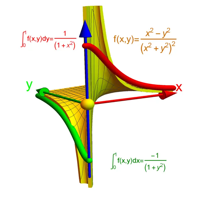
Without continuity, Fubini is false: the standard example is illustrated in Figure (22.3): \[\begin{aligned} \frac{-\pi}{4}=\int_{0}^{1} \int_{0}^{1} \frac{(x^{2}-y^{2})}{(x^{2}+y^{2})^{2}} \,d y \,d x \neq \int_{0}^{1} \int_{0}^{1} \frac{(x^{2}-y^{2})}{(x^{2}+y^{2})^{2}} \,d x \,d y=\frac{\pi}{4}. \end{aligned}\]
Proof. \[\begin{aligned} \int\frac{x^{2}-y^{2}}{(x^{2}+y^{2})^{2}} \,d x &= -\frac{x}{x^{2}+y^{2}},\\ \int\frac{x^{2}-y^{2}}{(x^{2}+y^{2})^{2}} \,d y &= \frac{y}{x^{2}+y^{2}}. \end{aligned}\] So that \[\begin{aligned} \int_{0}^{1} \frac{x^{2}-y^{2}}{(x^{2}+y^{2})^{2}} \,d x=-\frac{1}{1+y^{2}} \end{aligned}\] and \[\begin{aligned} \int_{0}^{1} \frac{x^{2}-y^{2}}{x^{2}+y^{2})^{2}} \,d y = \frac{1}{1+x^{2}}. \end{aligned}\] ◻
22.2.4 Multi-Index Notation and Higher Dimensional Integrals
Integrals in higher dimensions are defined in the same way. We will cover the three dimensional case in particular later. Lets just add the definition for now. Given a \(m\) dimensional region \(R\) in \(\mathbb{R}^{m}\) and a continuous \(f: \mathbb{R}^{m} \rightarrow \mathbb{R}\), using the multi-index notation \[x=(x_{1}, \ldots, x_{m}), \quad d x=d x_{1} \ldots d x_{m}, \quad \text{and} \quad i / n=(i_{1} / n, \ldots, i_{m} / n)\] define \[\int_{R} f(x) \,d x=\lim _{n \rightarrow \infty} \frac{1}{n^{m}} \sum_{\frac{i}{n} \in R} f\Big(\frac{i}{n}\Big).\] A region is now a set \[R=\left\{x \in \mathbb{R}^{m} \mid g_{1}(x) \leq c_{1}, \ldots, g_{k}(x) \leq c_{k}\right\}\] where \(g_{k}\) are smooth functions. It is called bounded if there exists \(\rho>0\) such that \(R \subset\{|x| \leq \rho\}\).
22.3 EXAMPLES
Example 1. If \(f(x, y)=1\), then \(\iint_{R} f(x, y) \,d x \,d y\) is the area of \(R\). For example, if \[\begin{aligned} \iint_{x^{2}+y^{2} \leq 9} 8 \,d x \,d y&=8 \iint_{x^{2}+y^{2} \leq 9} 1 \,d x \,d y\\ &=8 \mathrm{Area}(R)\\ &=72 \pi. \end{aligned}\]
Example 2. We know from single variable calculus that \(\int_{a}^{b} f(x) \,d x\) is the signed area under the curve of \(f\). For \(f(x) \geq 0\), where it is the area, we can write this as \(\int_{a}^{b} \int_{0}^{f(x)} 1 \,d y \,d x\). Note that as we have defined the integrals, the equivalence would be wrong if \(f(x)\) is negative somewhere. It is the double integral which is the correct notion of area. For exmaple, the area of the region bounded by the curve \(y=1 /(1+x^{2})\), the curve \(y=0\), the curve \(x=-1\), and \(x=1\) is \[\int_{-1}^{1} \int_{0}^{1 /(1+x^{2})} \,d y \,d x=\arctan(x)\big|_{-1} ^{1}=\pi / 2.\]
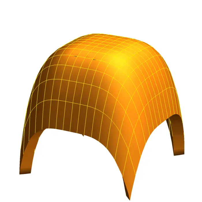
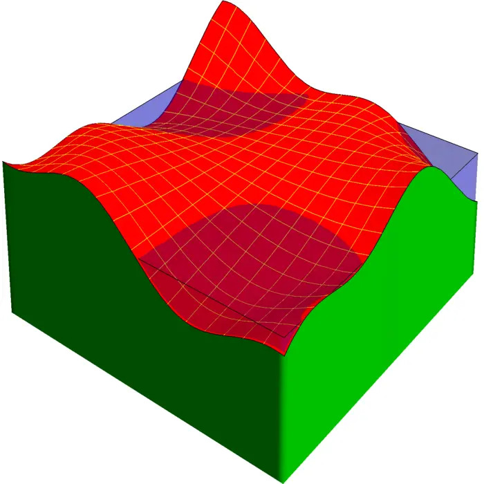
Example 3. Problem: The integral \(\iint_{R} f(x, y) \,d x \,d y\) can be interpreted as the signed volume under the graph of \(f\) above the region \(R\). Find the volume of the region bound by \(z= 4-2 x^{4}-2 y^{4}\) and \(z=4-2 x^{2}-2 y^{2}\) and \(-1 \leq x \leq 1\) and \(-1 \leq y \leq 1\).
Solution: \[\int_{0}^{1} \int_{0}^{1}\big((4-2 x^{4}-2 y^{4})-(4-2 x^{2}-2 y^{2})\big) d x \,d y=(4 / 15)^{2}.\]
Example 4. Problem: Find the area of a disc of radius \(a\).
Solution: \[\int_{-a}^{a} \int_{-\sqrt{a^{2}-x^{2}}}^{\sqrt{a^{2}-x^{2}}} 1 \,d y \,d x=\int_{-a}^{a} 2 \sqrt{a^{2}-x^{2}} \,d x.\] Use trig substitution \(x=a \sin (u)\), \(d x=a \cos (u)\), to get \[\int_{-\pi / 2}^{\pi / 2} 2 \sqrt{a^{2}-a^{2} \sin ^{2}(u)} \,a \cos (u) \,d u=\int_{-\pi / 2}^{\pi / 2} 2 a^{2} \cos ^{2}(u) \,d u\] Using a double angle formula, this gives \(a^{2} \int_{-\pi / 2}^{\pi / 2} 2 \,\frac{1+\cos (2 u)}{2} \,d u=a^{2} \pi\). We will next time compute this much more effectively.
Example 5. Problem: Let \(R\) be the triangle \(\{1 \geq x \geq 0,\ 0 \leq y \leq x\}\). Evaluate \(\iint_{R} e^{-x^{2}} \,d x \,d y\).
Solution: We can not evaluate the integral directly because \(e^{-x^{2}}\) has no anti-derivative given in terms of elementary functions. But we can write the integral as \(\int_{0}^{1}\left[\int_{0}^{x} e^{-x^{2}} \,d y\right] d x\): \[\begin{aligned} \int_{0}^{1}\left[\int_{0}^{x} e^{-x^{2}} \,d y\right] d x &=\int_{0}^{1} x e^{-x^{2}} \,d x\\ &=-\frac{e^{-x^{2}}}{2}\Big|_{0} ^{1}\\ &=\frac{1-e^{-1}}{2}. \end{aligned}\]
EXERCISES
Exercise 1. Calculate the iterated integral \(\int_{0}^{1} \int_{x}^{2-x}(x^{3}-y) \,d y \,d x\) in two ways, once as a "left to right" and once as a "bottom to top" integral.
Exercise 2. Find the integral \[\int_{0}^{1} \int_{\sqrt{y}}^{y^{2}} \frac{3 x^{7}}{\sqrt{x}-x^{2}} \,d x \,d y.\]
Exercise 3.
- Compute the area of the elliptical region bound by the ellipse \(x^{2} / 4^{2}+y^{2} / 9^{2}=1\) using trig substitution.
- Now do this in general for an ellipse \(x^{2} / a^{2}+y^{2} / b^{2}=1\).
(It is the "hardest problem in geometry", according to the comedy-drama "Rushmore", a movie from 1998).
Exercise 4. Find the integral \[\int_{0}^{\pi^{2}} \int_{\sqrt{y}}^{\pi} \frac{\sin (x)}{x^{2}} \,d x \,d y.\]
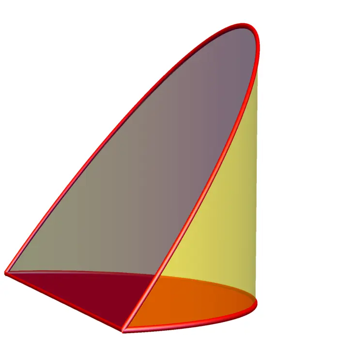
Exercise 5. Find the volume of the hoof solid \(x^{2}+y^{2} \leq 1\), \(0 \leq z \leq x\). The hoof solid was considered by Archimedes already.
Appendix: Data illustration: Monte Carlo
22.3.1 Lebesgue Integrals: A Tool for Real-World Integration
Often, when we deal with real data, we do not have analytic expressions for the region or function we want to integrate. The Riemann integral has its limitations. In other branches of mathematics like in probability theory, a better integral is needed. Its definition is close to the Riemann integral which we have given as the limit \(\int_{(x_{k}, y_{l}) \in R} f(x_{k}, y_{l}) \frac{1}{n^{2}}\), where \(x_{k}=k / n\), \(y_{l}=l / n\). The Lebesgue integral replaces the regularly spaced \((x_{k}, y_{l})\) grid with random points \((x_{k}, y_{l})\) and uses the same formula.
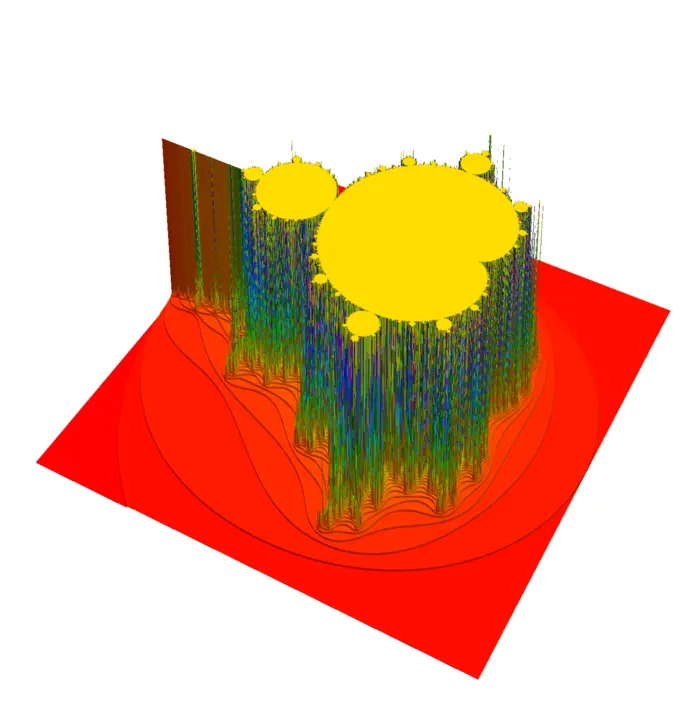
22.3.2 The Area of a Fractal
How do we find the area of Mandelbrot set \[M=\left\{c=a+i b \in \mathbb{C} \mid T_{c}(0)^{n} \text { stays bounded}\right\},\] where \(T_{c}(z)=z^{+} c\)? In real coordinates, this is the map \(T_{c}(x, y)=(x^{2}-y^{2}+a, 2 x y+b)\).
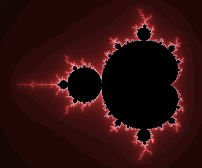
22.3.3 A Computational Approach to Mandelbrot Set Area
What is the area of the Mandelbrot set? We know it is contained in the rectangle \(x \in [-2,1]\) and \(y \in [-3 / 2,3 / 2]\). We now just randomly shoot into this rectangle and see whether we are in the Mandelbrot set or not after \(1000\) iterations. Here is some Mathematica code which allows you to compute things. When we ran it, it gave a value of about \(1.515\ldots\). More accurate measurements reported hint for a slightly smaller value like \(1.506\ldots\). Others have given bounds \([1.50311, 1.5613027]\).