Discrete Vector Calculus
Table of Contents
33.1 INTRODUCTION
33.1.1 Discrete Calculus
In this seminar as well as the one next week, we redo calculus on finite networks. This is how multi-variable calculus of the future might look like. There is no infinity, there are no limits. The mathematics is the same. We will formulate first the fundamental theorem of line integral, Green and Stokes theorem \(\int_{G} \,d F=\int_{d G} F\) on such a world.
33.1.2 Network Calculus
A finite network is a graph \((V, E)\), where \(V\) is a finite set of nodes called vertices and where \(E\) are connections between nodes. There are no loops in that connections connect different nodes and also, there is only one connection possible between two points. One calls \((V, E)\) a finite simple graph. Now similarly as we introduce coordinate systems in our space telling what is north, south, up or down, etc, we assign when doing computations an orientation on the edges. This is pretty arbitrary but usually done any way when we implement a graph on a computer. For example \[(G, V)=\big(\{1,2,3,4\},\{(1,2),(1,3),(1,4),(2,3),(2,4),(3,4)\}\big)\] is a graph with \(4\) nodes, where all nodes are connected to each other. When doing calculus, we look at functions on nodes, functions on edges, functions on triangular sugraphs as well as functions on tetrahedral subgraphs.
33.2 SEMINAR
33.2.1 Network Fields and Gradients
In this seminar, we replace the space \(\mathbb{R}^{n}\) with a finite graph \(G=(V, E)\), where \(V\) is a set of vertices called nodes and \(E\) is a set of edges called connections. A scalar field is a function \(f\) which assigns to every vertex \(x\) a function value \(f(x)\). We assume the vertices to be ordered leading to an order of the edges: draw an arrow \(a \rightarrow b\) if \(a
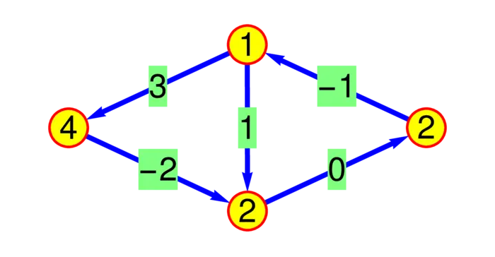
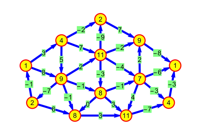
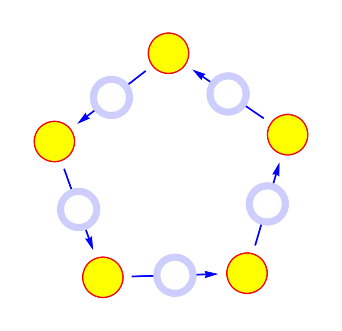
Problem A: Check the closed loop property of the gradient field \(\nabla f\) shown in the graph of Figure (33.2).
33.2.2 Discrete Line Integral Theorem
The discrete fundamental theorem of line integrals is:
Theorem 1. If \(F=\nabla f\) is a gradient field and \(C\) is a curve from \(a\) to \(b\), then \(\int_{C} \nabla f \cdot d r=f(b)-f(a)\).
Problem B: Prove the discrete fundamental theorem of line integrals by induction on the length of the curve \(C\).
33.2.3 Unit Spheres
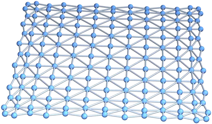
Let’s look at some terminology. Given a vertex \(x\) in a graph \(G\), the unit sphere \(S(x)\) of \(x\) is the sub-graph generated by the set of vertices directly attached to \(x\). The unit sphere of the vertex labeled \(11\) in Figure (33.3) for example is the circular graph generated by the vertices \(\{2,4,9,8,7,9\}\). It is a "circle". The unit sphere of the vertex with label \(4\) in that figure is the graph generated by the vertices \(\{11,7,1\}\). It is an linear graph, a half circle.
33.2.4 Discrete Regions
A graph is called a discrete two-dimensional region, if every unit sphere \(S(x)\) is a circular graph with \(4\) or more vertices or a linear graph with \(2\) or more vertices. The set of vertices for which the unit sphere is circular form the interior of the region. The other vertices form the boundary of the region. A two dimensional region without boundary is called closed. In Figure (33.3) for example, there are \(4\) interior points and \(9\) boundary points. In Figure (33.5), we see a closed region.
33.2.5 Discrete Curl
The curl of a vector field \(F\) is a function on the triangles \(T\) of \(G\). To get the value of the triangle \((a, b, c)\) we form the line integral of \(F\) along the curve \[C: a \rightarrow b \rightarrow c \rightarrow a.\] Each triangle is assumed to be oriented (if drawn in the plane, then counter clockwise).
33.2.6 Discrete Flux
Given a function \(F\) on the triangles of a region \(G\) which is oriented, the flux integral \(\iint_{G} F(x) \,d A\) is defined as \(\sum_{t \in T} f(t)\), where \(T\) is the set of triangles in \(G\).
33.2.7 Discrete Green’s Theorem
Here is the discrete Green’s theorem:
Theorem 2. If \(F\) is a vector field on a \(2\)-dimensional discrete region \(G\), and the boundary \(C\) is oriented in a compatible way with the region, then \[\iint_{G} \operatorname{curl}(F) \,d A=\int_{C} F \cdot d r.\]
33.2.8 Applying Green’s Theorem: Curl, Flux, and Verification
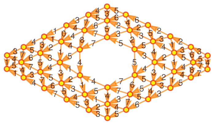
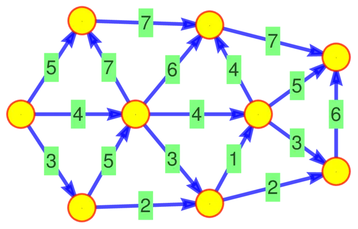
Figure (33.4) shows a region equipped with a vector field \(F\).
Problem C: Write in the curl of the vector field in Figure (33.4).
Problem D: Prove the discrete Green theorem by induction on the number of triangles.
EXERCISES
Exercise 1. Check that the curl of a gradient field is zero: \(\operatorname{curl}(\operatorname{grad}(f))=0\) for a general triangle: draw an oriented triangle. Define \(F=\nabla f\) for a scalar function \(f\), \(1\) then compute \(\operatorname{curl}(F)\).
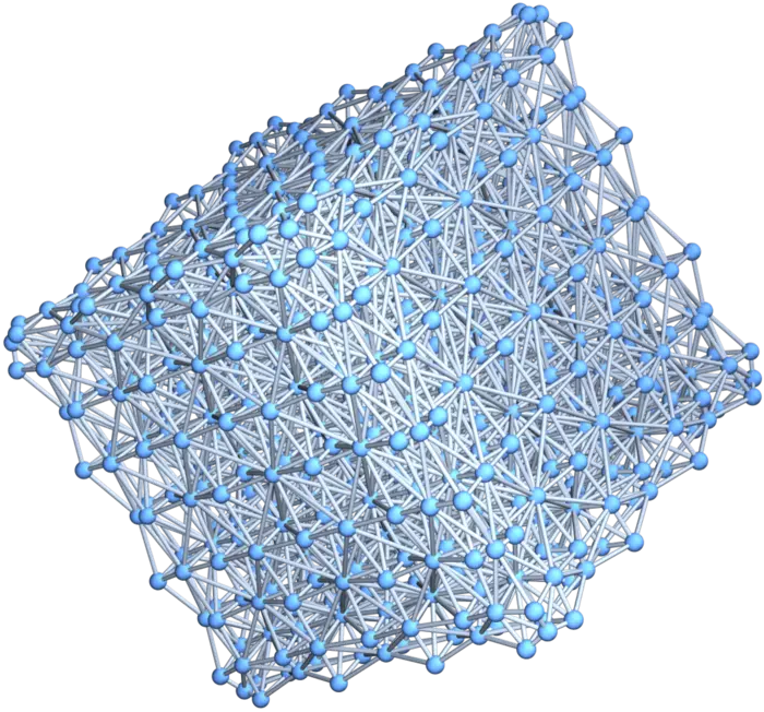
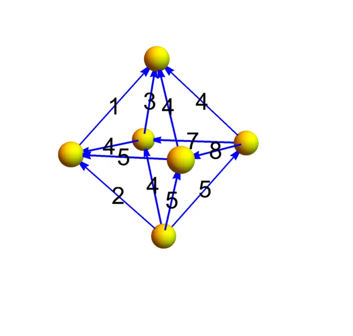
Exercise 2. Figure (33.5) shows a vector field on the octahedron a two dimensional discrete sphere. Determine all the curls and check that the sum of all curls is zero. You have checked \(\int_{S} \operatorname{curl}(F) \,d S=0\) for a closed surface.
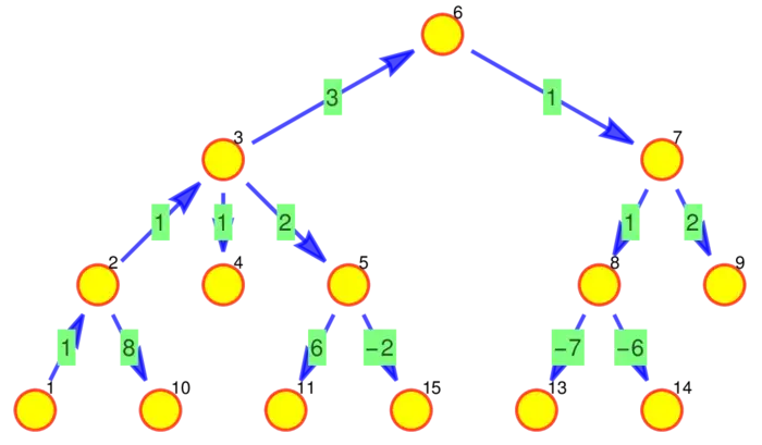
Exercise 3. Figure (33.6) shows a tree, a graph without closed loops. Find a potential function \(f\). You can assume that the value at the top node is \(0\). You see then that the function value right below is \(1\). Get all the function values of the potential.
Exercise 4. Find a vector field on a circular graph with \(5\) vertices which is not a gradient field.
Exercise 5. Check Green’s theorem in the following annular region. Compute both the line integral \(\int_{C} F \,d r\) along the boundary (which has two components) as well as \(\iint_{G} \operatorname{curl}(F) \,d A\), the sum of the curvatures over all triangles.