Curves
Table of Contents
- 7.1 INTRODUCTION
- 7.2 LECTURE
- 7.2.1 Parametrized Curves and Their Paths
- 7.2.2 Velocity and Acceleration on Curves
- 7.2.3 The Fundamental Theorem of Calculus and Curves
- 7.2.4 Tangent, Normal, and Binormal Vectors
- 7.2.5 Curvature Singularities and Smoothness
- 7.2.6 Concavity Changes and Normal Vectors
- 7.2.7 Side Remark: Matrix-Valued Curves
- 7.2.8 Side Remark: Simple Closed Curves
- 7.2.9 Side Remark: Constant Speed Reparametrization
- 7.2.10 Side Remark: Complexities of Continuous Curves
- 7.3 EXAMPLES
- EXERCISES
7.1 INTRODUCTION
7.1.1 Curves in Linear Algebra
Many geometric objects can be assigned a dimension. This number tells how many parameters we need to describe the object. A point has dimension \(0\), a line has dimension \(1\), a plane has dimension \(2\). This is formalized in linear algebra. Given a matrix \(A\), the number of leading \(1 \operatorname{in} \operatorname{rref}(A)\) is the dimension of the image of \(A\). The number of free variables (columns without leading \(1\) in \(\operatorname{rref}(A)\) is the dimension of the kernel of \(A\). For example, for \(A=[1,2,3]\) which is already in row reduced form, we have one leading \(1\) and two free variables \(y\) and \(z\). The equation \(1 {x}+2 {y}+3{z}=0\) describes a \(2\) dimensional object, a plane. If \(y, z\) are given, we can find \(x\) from the equation. The image of the column vector \(v=A^{T}\) is the line spanned by this vector. This line is perpendicular to the plane and illustrates the fundamental theorem of linear algebra assuring the kernel of \(A\) being perpendicular to the image of \(A^{T}\) or equivalently the kernel of \(A^{T}\) being perpendicular to the image of \(A\).
7.1.2 Dimensionality and Curves
Curves are objects of dimension \(1\). For example, the line spanned by a vector \(v\) is written as the set of points \(r(t)=t v=[t, 2 t, 3 t]^{T}\). We call this a parametrization of the line. The free variable \(t\) is called time. It determines, where we are located at a fixed time \(t\). At time \(t=12\) for example we are positioned at the point \((12,24,36)\) corresponding to the vector \([12,24,36]^{T}\).1 The vector \(v\) has the interpretation of a velocity. It tells us how fast we move on the line. Of course, replacing \(v\) with \(3 v\) would give us the same line but we would travel three times faster and would reach the point \((12,24,36)\) three times faster.
7.1.3 Exploring Curves in Space
If the velocity can change direction and length, we can drive around on more interesting paths. The frame work is to take three continuous functions \(x(t), y(t), z(t)\) and look at the path \((x(t), y(t), z(t))\) in space. We write this in vector notation as \(r(t)=[x(t), y(t), z(t)]^{T}\). Now, because we get tired always to write the \({T}\) pointing out that we use column vectors, we will just write \(r(t)=[x(t), y(t), z(t)]\). Most of the time, we assume the functions to be differentiable but the case of a ping-pong ball bouncing off a table shows that also non-smooth curves can matter even in daily life. Curves can be very complicated. Take a ping-pong ball and place it into an elliptic container. The billiard path it traces is chaotic. In this lecture we look at curves given by parameterizations, learn how to take derivative to get the velocity or acceleration. We also learn how to integrate. This allows us to compute paths. We can for example compute where a ball falling in a gravitational field is at time \(t\).
7.2 LECTURE
7.2.1 Parametrized Curves and Their Paths
Given \(n\) continuous functions \(x_{j}(t)\) of one variable \(t\), we can look at the vectorvalued function \(r(t)=\left[x_{1}(t), \ldots, x_{n}(t)\right]^{T}\). We call it a parametrized curve. An example is \(r(t)=[3+2 t, 4+6 t]\) which is a line through the point \((3,4)\) and containing the vector \([2,6]\).2 If \(t\) is in the parameter interval \(a \leq t \leq b\), then the image of \(r\) is \(\{r(t) \mid a \leq t \leq b\}\), which defines a curve in \(\mathbb{R}^{n}\). The curve starts at the point \(r(a)\) and ends at the point \(r(b)\). An other important example is the circle \(r(t)=[\cos (t), \sin (t)]\), where \(t\) is in the interval \([0,2 \pi]\). Its image is a circle in the plane \(\mathbb{R}^{2}\). The parametrization \(r(t)\) contains more information than the curve itself: the parabolic curve \(r(t)=[t, t^{2}]\) defined on \(t \in[-1,1]\) for example is the same as the curve \(r(t)=[t^{3}, t^{6}]\) for \(\in[-1,1]\), but in the second parametrization, the curve is traveled with different speed. Curves in \(\mathbb{R}^{3}\) can be admired in our physical space like \(r(t)=[x(t), y(t), z(t)]=[t \cos (t), t \sin (t), t]\) which is a spiral. This particular curve is contained in the cone \(x^{2}+y^{2}=z^{2}\).
7.2.2 Velocity and Acceleration on Curves
If the functions \(t \rightarrow x_{j}(t)\) are differentiable, we can form the derivative \[r^{\prime}(t)=\left[x_{1}^{\prime}(t), \ldots, x_{n}^{\prime}(t)\right].\] While this technically is again a curve, we think of \(r^{\prime}(t)\) as a vector attached to the point \(r(t)\) and say that \(r^{\prime}(t)\) is tangent to \(r(t)\). The length \(\left|r^{\prime}(t)\right|\) of the velocity is called the speed of \(r\). If also higher derivatives of the functions \(x_{j}(t)\) exist, we can form the second derivative \(r^{\prime \prime}(t)\) called the acceleration or third derivative \(r^{\prime \prime \prime}(t)=r^{(3)}(t)\) called the jerk. Then come snap \(r^{(4)}(t)\), crackle \(r^{(5)}(t)\) and pop \(r^{(6)}(t)\) and the Harvard \(r^{(7)}(t)\) introduced in the fall of 2016 in a multi-variable exam.
7.2.3 The Fundamental Theorem of Calculus and Curves
Given the first derivative function \(r^{\prime}(t)\) as well as the initial point \(r(0)\), we can get back the function \(r(t)\) thanks to the fundamental theorem of calculus. Because of Newton’s law which tells that a mass point of mass \(m\) subject to a force field \(F\) depending on position and velocity satisfies the Newtonian differential equation \(m r^{\prime \prime}(t)=F\left(r(t), r^{\prime}(t)\right)\), the following result is important:
Theorem 1. \(r(t)\) is uniquely determined from \(r^{\prime \prime}(t)\) and \(r(0)\) and \(r^{\prime}(0)\).
Proof. In each coordinate we get \[x_{k}^{\prime}(t)=\int_{0}^{t} x_{k}^{\prime \prime}(s)\,ds + x_{k}^{\prime}(0)\quad \text{ and }\quad x_{k}(t)=\int_{0}^{t} x_{k}^{\prime}(s)\,ds+x_{k}(0).\] We have just applied twice the fundamental theorem of calculus. ◻
A special case is if \(r^{\prime \prime}(t)\) is constant. A special case is the free fall situation. The coordinate functions are then quadratic. Assume \(r^{\prime \prime}(t)=[0,0,-10]\), and \(r^{\prime}(0)=[0,0,0]\) and \(r(0)=[0,0,20]\), then \(r(t)=[0,0,20-5 t^{2}]\). If you jump from \(20\) meters into a pool, you need \(t=2\) seconds to hit the water.
7.2.4 Tangent, Normal, and Binormal Vectors
Given a curve \(r(t)\) for which the velocity \(r^{\prime}(t)\) is never zero, we can form the unit tangent vector \(T(t)=r^{\prime}(t) /|r^{\prime}(t)|\). If \(T^{\prime}(t)\) is never zero, we can then form \(N(t)=T^{\prime}(t) /|T^{\prime}(t)|\), the normal vector. The vector \(B=T \times N\) is called the binormal vector. The scalar \(|T^{\prime}(t)| /|r^{\prime}(t)|\) is called the curvature of the curve.
Theorem 2. In \(\mathbb{R}^{3}\), we have \(K=|T^{\prime}| /|r^{\prime}|=|r^{\prime} \times r^{\prime \prime}| /|r^{\prime}|^{3}\).
Proof. We will do this computation in class. ◻
7.2.5 Curvature Singularities and Smoothness
Even if \(r(t)\) is perfectly smooth, the curvature can become infinite. Lets look at the example \(r(t)=[t^{2}, t^{3}, 0]\). Then \(r^{\prime}(t)=[2 t, 3 t^{2}, 0]\) and \(r^{\prime \prime}(t)=[2,6 t, 0]\) and \(r^{\prime}(t) \times r^{\prime \prime}(t)=[0,0,6 t^{2}]\). The curvature is \((6 / t)(4+9 t^{2})^{-3 / 2}\) which has a singularity at \(t=0\).
7.2.6 Concavity Changes and Normal Vectors
Even when \(r(t)\) is perfectly smooth and never zero, the normal vector can depend in a discontinuous way on \(t\). Example: \(r(t)=[t, t^{3} / 3]\). Now \(r^{\prime}(t)=[1, t^{2}]\) and \(T(t)=\) \([0, t^{2}] / \sqrt{1+t^{4}}\). We see that \(T^{\prime}(t)\) takes different signs in the second coordinate. After normalization we have \(\lim _{t \rightarrow 0, t>0} N(t)=[0,1]\) and \(\lim _{t \rightarrow 0, t<0} N(t)=[0,-1]\). At the inflection point of the graph of the cube function, the concavity has changed from concave down to concave up. This has changed the direction of the normal vector \(N\).
7.2.7 Side Remark: Matrix-Valued Curves
We have looked at parametrized vectors only. If the entries \(A_{i j}(t)\) of a matrix depend on times we have a matrix valued curve \(A(t)\). This appears in differential equations, in quantum mechanics (operators moving in time) or –most importantly– in moving pictures! A movie is just a matrix valued curve.
7.2.8 Side Remark: Simple Closed Curves
A planar curve \(r(t)=[x(t), y(t)]^{T}\) in the plane defined on \(t \in[0,2 \pi]\) is called a simple closed curve if \(r(0)=r(2 \pi)\) and there are no values \(0 \leq s \neq t<2 \pi\) for which \(r(t)=r(s)\). For a smooth curve, meaning that the first two derivatives exist, we can look at the polar angle \(\alpha(t)\) of the vector \(r^{\prime}(t)\). Define the signed curvature of the curve as \(\kappa(t)=\alpha^{\prime}(t) /|r^{\prime}(t)|\). We have \(|\kappa(t)|=K(t)\). The Hopf Umlaufsatz tells \(\int_{0}^{2 \pi} \kappa(t) d t=2 \pi\). In the case of the circle for example, \(\kappa(t)=1\).
7.2.9 Side Remark: Constant Speed Reparametrization
We can verify that any curve \(r(t)\) parametrized on \([a, b]\) such that \(r^{\prime}(t) \neq 0\) for all \(t \in[a, b]\) can be parametrized as \(R(t)\) on \([a, b]\) such that \(|R^{\prime}(t)|=1\) for all \(t\).
Proof: we look for a monotone function \(s(t)\) such that the derivative of \(r(s(t))\) has length \(1\). This means we want \(|r^{\prime}(s(t))| s^{\prime}(t)=1\). In other words, look for a function \(s(t)\) such that \(s^{\prime}(t)=1 /|r^{\prime}(s(t))|=F(s(t))\) and \(s(a)=0\). This is what we call a differential equation. There is a general existence theorem for differential equations (proven later) which assures that there exists a unique solution \(s(t)\). End of proof.
The result is very intuitive. You can drive from \(r(a)\) to \(r(b)\) along the curve traced by \(r(t)\) by just keeping the speed \(1\). This gives your your new parametrization. Your new time interval will be \([0, L]\) where \(L\) is the arc length (the length of your trip). We will come to arc length computation in the next lesson.
7.2.10 Side Remark: Complexities of Continuous Curves
Continuous curves can be complicated: If you look at the pollen particle in a microscope, it moves erratically on a curve which is nowhere differentiable as it is constantly bombarded with air molecules which bounce it around. This is Brownian motion. There are also Peano curves or Hilbert curves \([0,1] \rightarrow[0,1]^{2}\) or space filling Hilbert curves \(r(t):[0,1] \rightarrow Q=[0,1]^{3}\) which cover every point of the cube \(Q\). These curves define a continuous bijection from \([0,1]\) to \([0,1]^{3}\). (The inverse is not continuous. Still, the construction shows that there are the same number of points in \([0,1]\) than in \([0,1]^{3}\)).
7.3 EXAMPLES
Example 1. Assuming the Newton equations \(m r^{\prime \prime}(t)=F(t)\), find the path \(r(t)\) of a body of mass \(m=1 / 2\) subject to a force \(F(t)=[\sin (t), \cos (t),-10]\) with \(r(0)=[3,4,5]\) and \(r^{\prime}(0)=[1,2,7]\).
Solution: we have \(r^{\prime \prime}(t)=[2 \sin (t), 2 \cos (t),-20]\). Integration gives \[r^{\prime}(t)=[-2 \cos (t), 2 \sin (t),-20 t]+\left[c_{1}, c_{2}, c_{3}\right].\] Fixing the constants gives \[r^{\prime}(t)=[3-2 \cos (t), 2+2 \sin (t), 7-20 t].\] A second integration gives \[r(t)=[3 t-2 \sin (t), 2 t-2 \cos (t), 7 t-10t^{2}]+\left[c_{1}, c_{2}, c_{3}\right]\] with other constants \(C=\left[c_{1}, c_{2}, c_{3}\right]\). Comparing \[r(0)=[0,-2,0]+\left[c_{1}, c_{2}, c_{3}\right]=[3,4,5]\] gives \[r(t)=\left[3+3 t-2 \sin (t), 6+2 t-2 \cos (t), 5+7 t-10 t^{2}\right].\]
Example 2. Let \(r(t)=[L \cos (t), L \sin (t), 0]\). Then \[r^{\prime}(t)=[-L \sin (t), L \cos (t), 0] \quad \text{and} \quad r^{\prime \prime}(t)= [-L \cos (t),-L \cos (t), 0]\] and \[r^{\prime}(t) \times r^{\prime \prime}(t)=\left[0,0, L^{2}\right] \quad \text{and} \quad \left|r^{\prime}(t)\right|=L.\] So that \(|r^{\prime}(t) \times r^{\prime \prime}(t)|/| r^{\prime}(t)|^{3}=1 / L\). A circle of radius \(L\) has curvature \(1 / L\)!
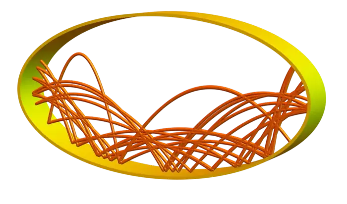
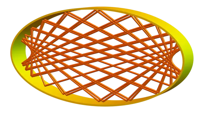
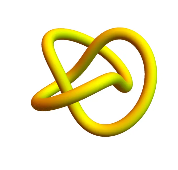
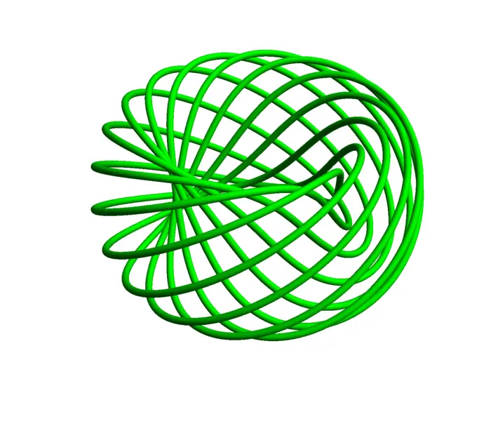
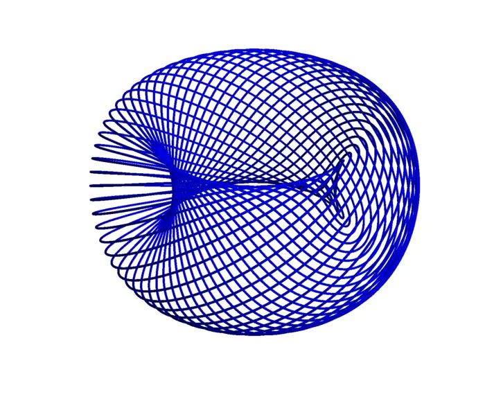
Example 3. A closed simple curve \(C\) in \(\mathbb{R}^{3}\) is a knot. For any positive integer \(n\), \(m\) we can look at the torus knot \[r(t)=\big[(3+\cos (m t))\cos (n t), (3+\cos (m t))\sin (n t), \sin (m t)\big].\] The total curvature of a knot is defined as \(\int_{0}^{2 \pi} K(t) \, dt\). See Figure (7.3).3
EXERCISES
Exercise 1. You sit on a bench at \(A=r(0)=[0,0,3]\) near the frozen Charles located between Winthrop and Elliot and chip stones aiming at \(B=[0,-300,15]\), a point near the Harvard business school. In order not to get into trouble, we assume everything happens in our imagination and that the stone is friction-free. You use a sling shot and throw with initial velocity \(r^{\prime}(0)=[0,-24,61]\), assume the gravitational acceleration to be \(r^{\prime \prime}(t)=[0,0,-10]\) at all times and use meters for distance and seconds for time. At which point does the stone reach the \(15\) meter height mark while descending? [Optional: you like a challenge and want to bounce off on the ice surface at \(C=[0,-200,0]\) and reach the point \(B\). What initial velocity \(v\) at \(A\) does achieve this?]
Exercise 2. We want to produce a logo for a new company and experiment. Draw the curve \(r(t)=[\cos (t), \sin (t)]+[\cos (11 t), \sin (9 t)] / 4\) and find the velocity, acceleration, and curvature at \(t=0\).
Exercise 3. Parametrize the curve \(r(t)\) obtained by intersecting the cylinder \(x^{2} / 9+y^{2} / 4=1\) with the plane \(z=x+5 y\).
Exercise 4. Verify that the torus knot \[r(t)=[x(t), y(t), z(t)]=\big[(2+\cos (m t))\cos (n t), (2+\cos (m t)) \sin (n t), \sin (m t)\big]\] lives on the torus \[(3+x^{2}+y^{2}+z^{2})^{2}-16(x^{2}+y^{2})=0.\]
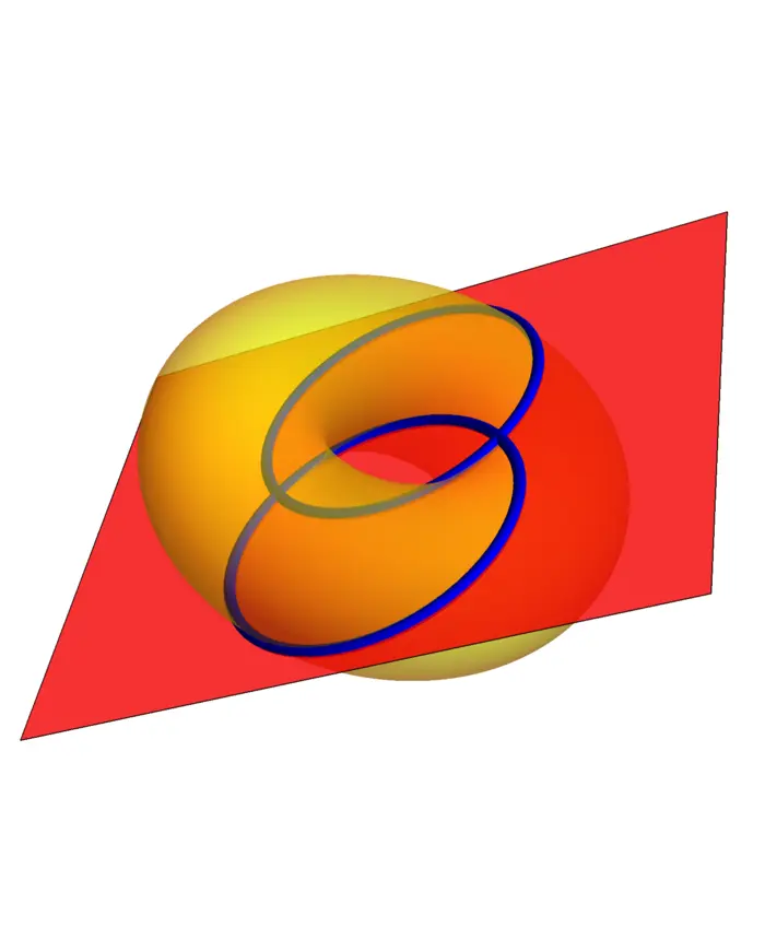
Exercise 5. You slice a bagel in a non-standard way. Let us assume that the bagel is given by \[(x^{2}+y^{2}+z^{2}+16)^{2}-100(x^{2}+y^{2})=0.\] Verify that if we intersect this torus with the plane \(3 x=4 z\), then we get the Villarceau circles \[r(t)=[4 \cos (t), 3+5 \sin (t), 3 \cos (t)]\] as well as the circle \[r(t)=[4 \cos (t),-3+5 \sin (t), 3 \cos (t)].\]
- We can associate any vector \({v}\) with a point. Think of the vector as connecting \(0\) with the point.↩︎
- To reduce clutter, we write row vectors \([2,6,1]\) rather than column vectors \([2,6,1]^{T}\).↩︎
- A general theorem of Fay and Milnor assures that a knot of total curvature \(\leq 4\pi\) is trivial.↩︎