Arc Length
Table of Contents
8.1 INTRODUCTION
8.1.1 Introduction to Arc Length
In this lecture we really get into calculus as we use both differentiation as well as integration to compute the length of curves. This unit is also a good point to brush up some integration techniques. The main theoretical result is that if \(r^{\prime}(t)\) is piecewise continuous, then we can compute the length. Mathematically we will see that the Riemann integral \(\int_{a}^{b} f(t)\, dt\) exists for every continuous function.
8.1.2 Calculus Foundations of Arc Length
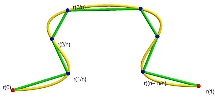
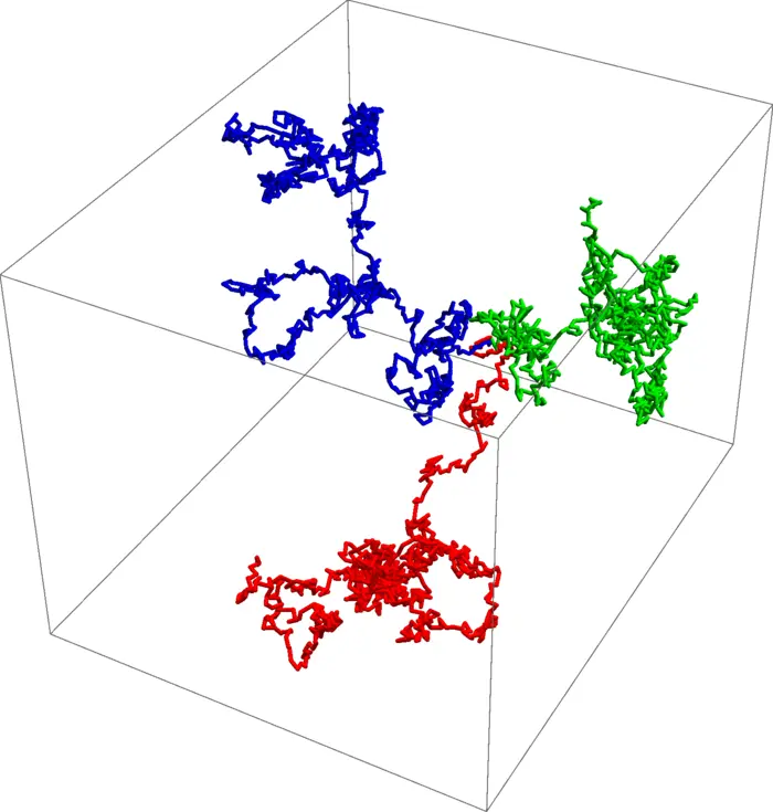
In single variable calculus courses, one usually assumes that \(f\) is differentiable in which case the proof is much simpler. So, in some sense, we want to illustrate here also that calculus leads to real analysis which is close also to the core foundations of mathematics. Both when computing derivatives or integrals we are using a notion of "limit". When we compute the length of a curve we split it into small pieces and add up the lengths of these pieces. That his process gives a limiting finite end result is by no means trivial. If we look at the motion of a pollen particle in a fluid and compute the length by tracking smaller and smaller time intervals, the length actually diverges to infinity.

8.2 LECTURE
8.2.1 Continuous Curves and Uniqueness of Parameterization
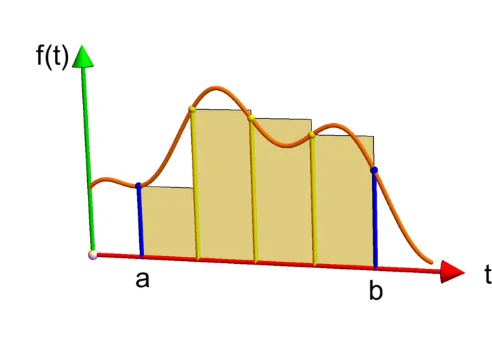
We assume in this lecture that curves are continuously differentiable meaning that the velocity is continuous. We would write \(r \in C^{1}([a, b], \mathbb{R}^{d})\). Given a parametrized curve \(r(t)\) defined over an interval \(I=[a, b]\), its arc length is defined as \[L=\int_{a}^{b}\left|r^{\prime}(t)\right| dt.\] For \(f(t)=\left|r^{\prime}(t)\right|\) the integral is defined as the lim sup (we don’t know yet whether lim exists), \[\int_{a}^{b} f(t)\,dt=\limsup _{n \rightarrow \infty} \frac{S_{n}}{n}=\limsup _{n \rightarrow \infty} \frac{1}{n} \sum_{a \leq \frac{k}{n}
Theorem 1. Arc length exists and is independent of the parameterization.
Proof.
- To see parameter independence, assume a time change \(\phi(t)\) with a monotone smooth function \(\phi:[a, b] \rightarrow[\phi(a), \phi(b)]\). If \(r(t)\) on \([\phi(a), \phi(b)]\) and \(R(t)=r(\phi(t))\) on \([a, b]\) are the two parametrizations and \[f(t)=|r^{\prime}(t)| \quad \text{and} \quad F(t)=|R^{\prime}(t)|=|r^{\prime}(\phi(t))| \phi^{\prime}(t),\] then by substitution, the arc length of \(r(t)\) is \[\int_{\phi(a)}^{\phi(b)} f(t)\, d t=\int_{a}^{b} f(\phi(t)) \phi^{\prime}(t)\, d t\] which is \(\int_{a}^{b} F(t)\, d t\), the arc length of \(R(t)\).
- From (i) we can assume \([a, b]=[0,1]\). By uniform continuity, there are \(M_{n} \rightarrow 0\) such that if \(|y-x| \leq 1 / n\), then \(|f(y)-f(x)| \leq M_{n}\). The intermediate value theorem, gives for every \[I_{k}=\left[x_{k}, x_{k+1}\right]=[k / n,(k+1) / n] \subset[0,1],\] a \(y_{k} \in I_{k}\) such that \(\int_{x_{k}}^{x_{k+1}} f(x)\, d x=f(y_{k}) / n\). Now, \(\int_{0}^{1} f(x)\, d x=(1 / n) \sum_{k} f(y_{k})\) and \[\begin{aligned} \left|S_{n} / n-\int_{0}^{1} f(x)\, d x\right|&=(1 / n)\Big|\sum_{k}\left[f(x_{k})-f(y_{k})\right]\Big|\\ &\leq(1 / n) \sum_{k}\left|f(x_{k})-f(y_{k})\right|\\ &\leq 1 / n \sum_{k} M_{n}\\ &=M_{n} \rightarrow 0. \end{aligned}\]
◻
8.3 EXAMPLES
Example 1. The arc length of the circle \(r(t)=[R \cos (t), R \sin (t)]\) with \(t \in[0,2 \pi]\) is \[\int_{0}^{2 \pi}|r^{\prime}(t)|\,d t=\int_{0}^{2 \pi} R\, d t=2 \pi R.\]
Example 2. The arc length of the parabola \(r(t)=[t, t^{2} / 2]\) with \(t \in[-1,1]\) is \(\int_{-1}^{1} \sqrt{1+t^{2}}\, d t\). We will do this integral in class. The result is \(\sqrt{2}+\operatorname{arcsinh}(1)\).
Example 3. The arc length of the curve \(r(t)=[\log (t), \sqrt{2} t, t^{2} / 2]\) for \(t \in[1,2]\). It is \[\int_{1}^{2} \sqrt{1 / t^{2}+t^{2}+2}\, d t=\int_{1}^{2}(t+1 / t)\, d t=\log (2)+3 / 2.\]
8.4 ILLUSTRATIONS
EXERCISES
Exercise 1. Find the arc length of the curve \[r(t)=[12 t, 8 t^{3 / 2}, 3 t^{2}],\] where \(t \in[0,7]\).
Exercise 2. Find the arc length of the cycloid \[r(t)=[t-\sin (t), 1+\cos (t)]\] from \(0\) to \(2 \pi\). The upside down cycloid is the solution to the famous Brachistochrone problem, the curve along which a ball descends fastest.
Hint. You might want to use the double angle formula \(2-2 \cos (t)=4 \sin ^{2}\big(\frac{t}{2}\big)\).
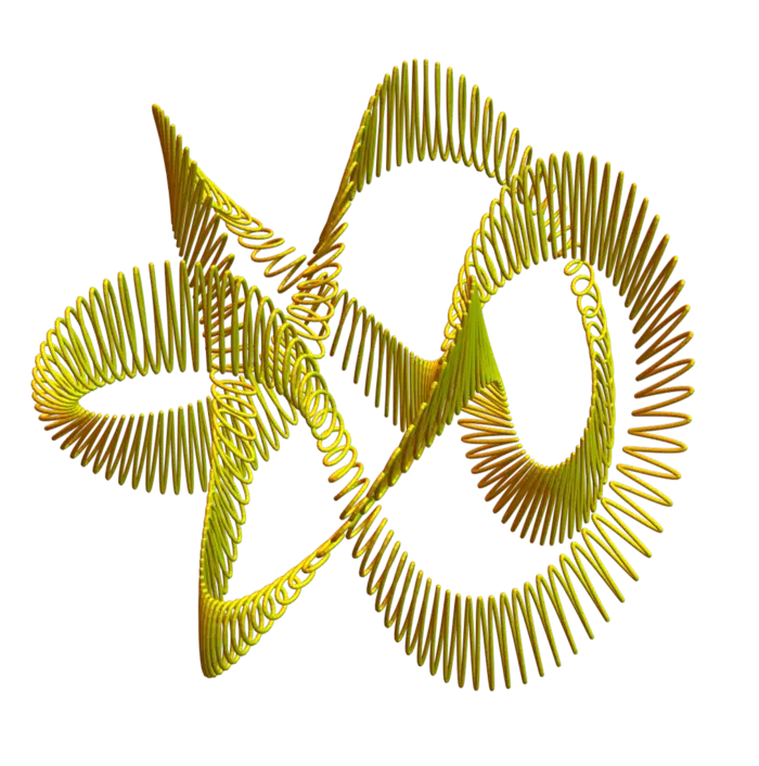
Exercise 3. Compute numerically the arc length of the knot \[r(t)=[\sin (4 t), \sin (3 t), \cos (5 t), \cos (7 t)]\] from \(t=0\) to \(t=2 \pi\). By drawing the first coordinates only and using color as the fourth coordinate, we can see that there are no non-trivial knots in \(\mathbb{R}^{4}\). You can not tie your shoes in \(\mathbb{R}^{4}\)!
Exercise 4. What is the relation between \(\left|\int_{0}^{1} r^{\prime}(t)\, d t\right|\) and \(\int_{0}^{1}\left|r^{\prime}(t)\right| d t\)? Give an interpretation of both sides.
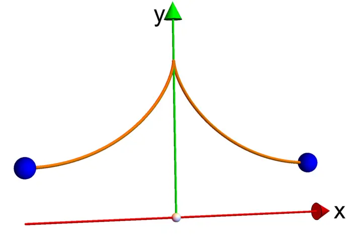
Exercise 5. Find the arc length of the catenary1 \(r(t)=[t, \cosh (t)]\), where \(\cosh (t)=\left(e^{t}+e^{-t}\right) / 2\) is the hyperbolic cosine and \(t \in[-1,1]\).
Hint. You can use the identity \(\cosh ^{2}(t)-\sinh ^{2}(t)=1\), where \(\sinh (t)=\) \(\left(e^{t}-e^{-t}\right) / 2\) is the hyperbolic sine. We have \(\cosh ^{\prime}=\sinh\), \(\sinh ^{\prime}=\cosh\).
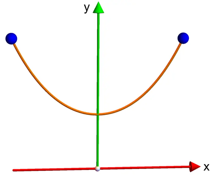
- Galileo was the first to investigate the catenary. It is the curve, a freely hanging heavy rope describes, if the end points have the same height. Galileo mistook the curve for a parabola. It was Johannes Bernoulli in 1691, who obtained its true form after some competition involving Huygens, Leibniz and two Bernoullis. The name "catenarian" (=chain curve) was first used by Huygens in a letter to Leibnitz in 1690.↩︎