A Discrete World
Table of Contents
36.1 INTRODUCTION
36.1.1 Fields, Forces, and Quantum Worlds
The Maxwell equations \[\fbox{$d F=0, d^{*} F=j$}\] allow to get the electro-magnetic field \(F\) from the current \(j\). The gravitational field is determined via the Gauss law \[\fbox{$d^{*} F=\rho$}\] from the mass density \(\rho\). With \(-\Delta=d^{*} d\), the Schrödinger equation \[\fbox{$i h u^{\prime}=-\Delta u+V u$}\] describes the motion of a quantum particles. On a space with a derivative \(d\), there is light, matter and a periodic system of atoms.
36.1.2 Laplacian Eigenvalues and Quantum Evolution
An important object in calculus is the Laplacian \(\Delta f=\operatorname{div}(\operatorname{grad}(f))\) which is \(\Delta f=f_{x x}+f_{y y}+f_{z z}\). For graphs, it is the Kirchhoff matrix \(K=d^{*} d\), where \(d^{*}\) is the transpose matrix of \(d\). The matrix \(K=d^{*} d\) is a square matrix with non-negative eigenvalues. Construct each column with \(K e_{v}\) where \(e_{v}\) is a basis vector. The \(1\)-form \(d e_{v}\) attaches to an edge connected to \(v\) the value \(-1\). Then \(d^{*} d e_{v}\) is the function on vertices which attaches to a vertex itself the negative of the vertex degree and to each attached node value \(1\). The Schrödinger equation \(i \hbar u^{\prime}=K u\) is solved by \[u(t)=U(t) u(0)=e^{-i t K / \hbar h} u(0).\] You can watch it with:
36.2 LECTURE
36.2.1 Graph Forms: Gradient, Curl, and Discrete Stokes
A \(\boldsymbol{0}\)-form \(f\) on a graph \(G=(V, E)\) is a function on the vertices \(V\). We also call it a scalar function. A \(\boldsymbol{1}\)-form is a function on the oriented edges \(E\) satisfying \(F(a, b)=-F(b, a)\). Informally, as in the continuum, we think of a \(1\)-form as a vector field. The gradient \[F(a, b)=d f(a, b)=f(b)-f(a)\] of a \(0\)-form \(f\) is a \(1\)-form \(F\). The curl of a vector field \(F\) is a \(\boldsymbol{2}\)-form. It is a function on triangles \((a, b, c)\) given by \[d F(a, b, c)=F(a, b)+F(b, c)+F(c, a)\] which can be seen as the line integral along the boundary of the triangle. When describing \(p\)-forms for \(p>0\), orientation matters. To fix it, just enumerate the vertices \(V\) and then choose the orientation of an edge \((a, b)\) with \(a
36.2.2 Discrete Divergence Theorem
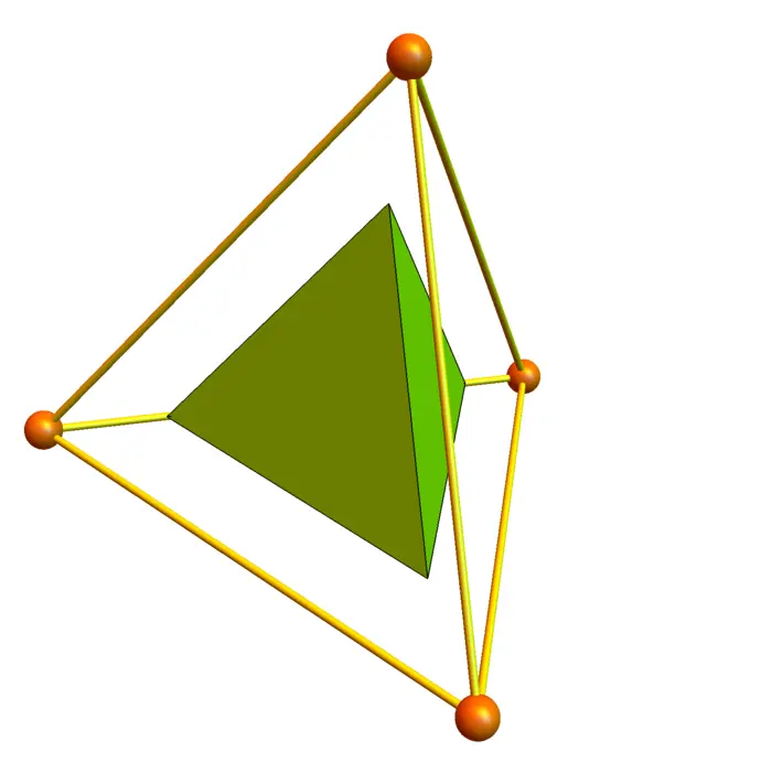
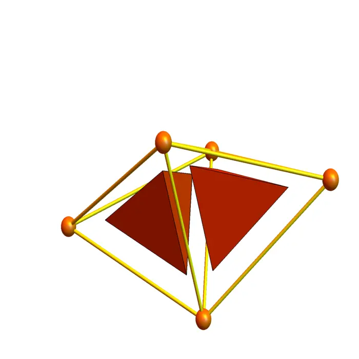
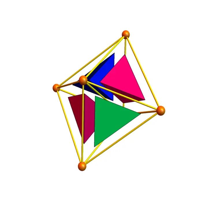
A tetrahedral graph is a collection of four nodes which all are connected to each other. A \(\boldsymbol{3}\)-form on a graph \(G\) is a function on tetrahedral sub-graphs \(x\) of \(G\). An example is the divergence \(\boldsymbol{d F(x)}\) of a \(\boldsymbol{2}\)-form \(\boldsymbol{F}\) which is defined as the sum of the \(F(y)\) values of the triangles \(y \subset x\) enclosing the tetrahedron \(x\). As in the continuum, the orientation plays a role. Here is the discrete divergence theorem for a solid \(G\) is built by tetrahedra \(x\) and where the boundary surface \(S\) consists of triangles:
Problem A: Check that \(\sum_{x \in G} \operatorname{div}(F)(x)=\sum_{y \in S} F(y)\).
Hint: prove by induction with respect to the number of tetrahedra. First check that if \(G\) is a single tetrahedron, this is the definition of the divergence. Then see what happens if a new tetrahedron is added.
36.2.3 Discrete Curl’s Vanishing Divergence
We also have seen that the divergence of the curl of a vector field \(F\) is zero: we had \[\operatorname{curl}(F)=[R_{y}-Q_{z}, P_{z}-R_{x}, Q_{x}-P_{y}]\] and taking the \(x\) derivative of \(R_{y}-Q_{z}\) is \(R_{y x}-Q_{z x}\), the \(y\) derivative of \(P_{z}-R_{x}\) is \(P_{z y}-R_{x y}\) and the \(z\)-derivative of \(Q_{x}-P_{y}\) is \(Q_{x z}-P_{y z}\). Adding them all up gives \(0\). In the discrete it is even simpler. Start with a \(1\)-form \(F\) on the edges of a graph. Then form the curls, which are functions on the triangles, then add up all these curls. You check:
Problem B: Check: \(\operatorname{div}(\operatorname{curl}(F))(x)=0\) of every \(F\) and tetrahedron \(x\).
36.2.4 p-Forms and Discrete Stokes
The general Stokes theorem is not much different. A \(\boldsymbol{p}\)-simplex in \(G\) in a complete sub-graph with \(p+1\) nodes. This means we have all connected to each other. A \(\boldsymbol{p}\)-form is a function on the set of \(p\)-simplices \(x\) in \(G\). The function value changes if two elements switch. For example, \[\begin{aligned} F(x_{0}, x_{1}, x_{2})&=F(x_{1}, x_{2}, x_{0})\\ &=F(x_{2}, x_{0}, x_{1})\\ &=-F(x_{1}, x_{0}, x_{2})\\ &=-F(x_{0}, x_{2}, x_{1})\\ &=-F(x_{2}, x_{1}, x_{0}). \end{aligned}\]
36.2.5 Discrete Exterior Derivative: Antisymmetry and Double Annihilation
The exterior derivative of \(p\)-form \(F\) is the \((p+1)\)-form \[d F(x_{0}, \ldots, x_{p+1})=\sum_{j=0}^{p+1}(-1)^{j} F(x_{0}, \ldots, \hat{x}_{j}, \ldots x_{p+1})\]
Problem C: Check in general that \(d d F=0\).
36.2.6 Stokes on Graphs: Integration by Parts
The general Stokes theorem tells that for a \(m\)-dimensional graph \(G\) with boundary \(S\) and a \((m-1)\)-form \(F\) we have
Theorem 1. \(\sum_{x \in G} d F(x)=\sum_{y \in S} F(y)\).
36.3 GRAVITY
36.3.1 Discrete Gravity and the Laplacian
The Newton equations \[\frac{d^{2}}{d t^{2}} x_{k}=-\sum_{j} G m_{j} /|x_{k}-x_{j}|^{2}\] with gravitational constant \(G\) describe the motion of finitely many mass points with positions \(x_{k}(t) \in \mathbb{R}^{3}\) and mass \(m_{k}\). These classical laws govern the motion of planets in our solar system, stars in a galaxy or galaxies in a galaxy cluster. While relativity modifies this Newtonian picture slightly and produces corrections which for example manifest in the perihelion advancement of Mercury, the Newtonian theory is amazingly accurate. Gauss derived the gravitational inverse square force \(F\) from \(\operatorname{div}(F)=4 \pi \sigma\), where \(\sigma\) is the mass density. While divergence usually maps a \(2\)-form to a \(3\)-form, it is the adjoint \(d^{*}\) of the gradient \(d\). In \(\mathbb{R}^{3}\) it is equivalent. Now, \[L=\operatorname{div} \circ \operatorname{grad}=d^{*} d: \Lambda^{0} \rightarrow \Lambda^{0}\] is called the Kirchhoff Laplacian. The Gauss law of gravity therefore is the Poisson equation \[\fbox{$L V=4 \pi \sigma$},\] where \(V\) is the gravitational potential, a \(0\)-form. Since \(d^{*}=0\) on \(0\)-forms, we can also write \(L=d d^{*}+d^{*} d\). Classical gravity gets from a mass density \(\sigma\) the gravitational potential \(V\) and so the gravitational field as a gradient \(F=d V\):
\((d^{*} d+d d^{*}) V=4 \pi \sigma\) defines the gravitational \(1\)-form \(F=d V\).
36.4 ELECTROMAGNETISM
36.4.1 Discrete Maxwell with Currents
The Maxwell equations \[\begin{aligned} \operatorname{div}(E)&=4 \pi \sigma,\\ \operatorname{div}(B)&=0,\\ \operatorname{curl}(E)&=-B_{t},\\ \operatorname{curl}(B)&=E_{t}+4 \pi i \end{aligned}\] become more elegant when written in four-dimensional space-time \(\mathbb{R}^{4}\). There are then two equations only. The first is \(d F=0\) which is evident from \(F=d A\) and \(d^{2}=0\). The second is \(d^{*} F=4 \pi j\), where \(j\) is the \(\boldsymbol{4}\)-current encoding both the charge density \(\sigma\) as well as the electric current \(i\). Now \(d F=0\) implies in a simply connected region that \(F=d A\), where \(A\) is an electro-magnetic potential. If \(d^{*} A=0\) (which can always be achieved by adding a gradient to \(A\)) we get the Poisson equation \[L A=(d d^{*}+d^{*} d) A=4 \pi j.\] This completely encodes the Maxwell equations; we can look at it also in a discrete network. Classical electromagnetism in a world with charge and current density \(j\) is the field \(F=d A\), where \(A\) is obtained from:
\((d^{*} d+d d^{*}) A=4 \pi j\) defines the electromagnetic \(2\)-form \(F=d A\).
36.5 QUANTUM MECHANICS
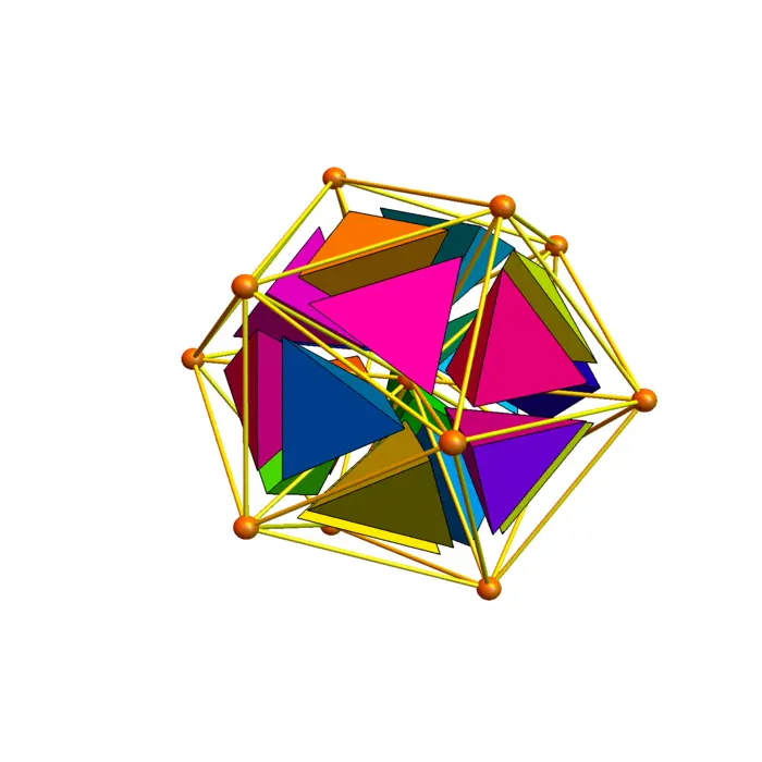
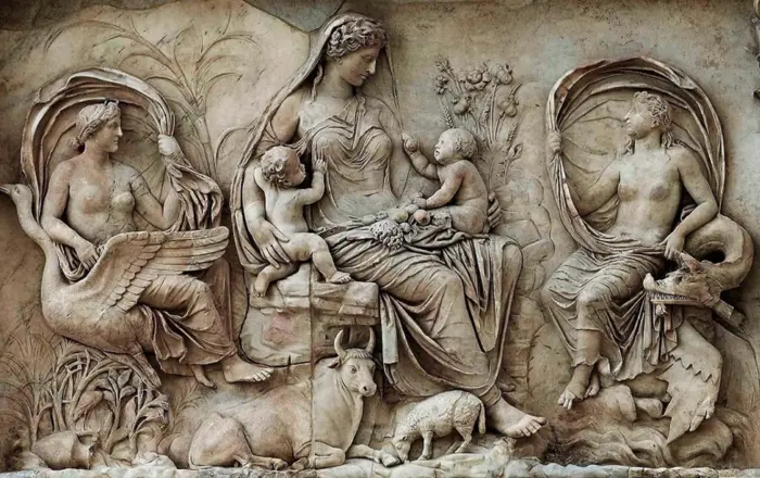
36.5.1 Discrete Quantum Field on Gaia
In this last homework we deal with a small universe \(G\). We call it Gaia, the primordial deity of earth. In Greek mythology, Gaia was the daughter of Aether the god of air and Hemera the goddess of light. We only create the gravitational field, the electromagnetic field on \(G\) and some quanta, so there will be matter and light in this world. But that mathematics is exactly as in the universe we live in: the classical gravitational field is described with the language of Gauss which we have seen to imply the Newton law of gravity. The electromagnetic field is formulated according to Maxwell, but directly in space-time. We also look a bit at quantum mechanics as the eigenvalues and eigenvectors of the Laplacian \(L\) play a role when looking at the Wheeler De Witt equation, a time-independent Schrödinger equation in space time
\((d^{*} d+d d^{*}) F=\lambda F\) defines a wave function \(F\) on \(p\)-forms.
36.5.2 Time Evolution on Discrete Lattices
The time dependent Schrödinger equation, as mentioned in the introduction can also be studied. For graphs, it is an ordinary differential equation.
36.6 BEYOND
36.6.1 From Quarks to Cosmos
The rest will be up to you: it remains to include the Fermionic constituents of matter (quarks (building mesons and baryons) as well as leptons) and bosons (photons, gluons, vector bosons and the Higgs) as well as a few other details called the Standard model. Don’t complain about the homework, a former \(22\)-student has solved a \(10^{222}\) node homework assignment in less than \(7\) days...
EXERCISES
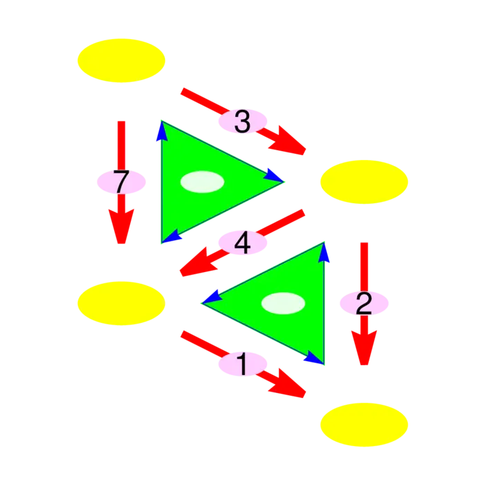
Exercise 1. Given the \(1\)-form \(F\) in Figure (36.4b), find the \(0\)-form \[f(x)=d^{*} F(x)=\sum_{e,\ e \rightarrow x} F(e).\] Check that \(\sum_{x \in V} d^{*} F(x)=0\). (This conservation law is a variant of the divergence theorem. (In the continuum, where \(2\)-forms and \(1\)-forms are identified and \(3\)-forms are equated with \(0\)-forms, this so called Kirchhoff law corresponds to the usual divergence theorem).
Exercise 2.
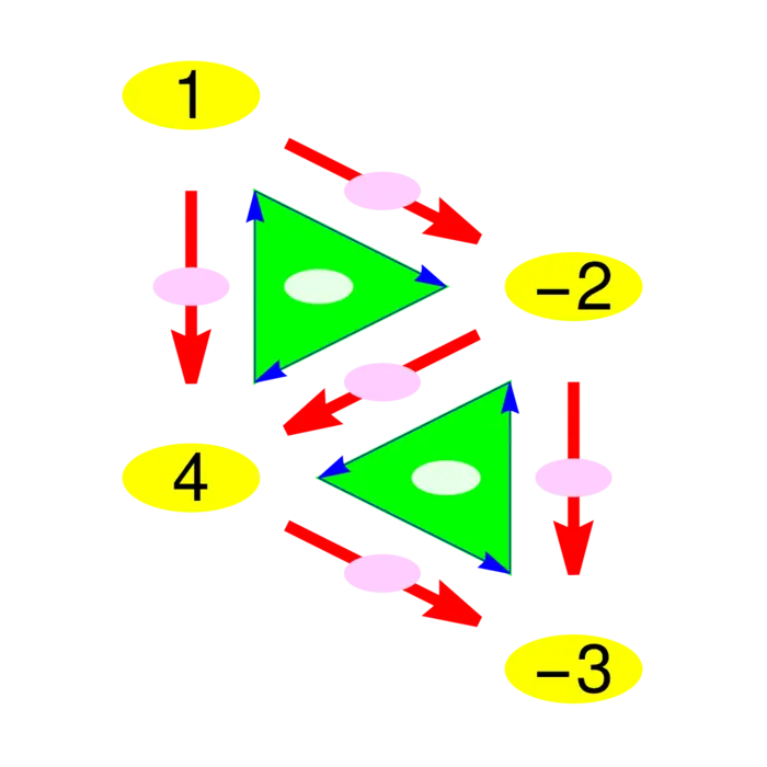
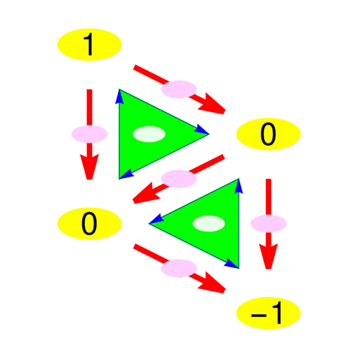
- Given the \(0\)-form \(f\) in Figure (36.4a), find \(F=d f\), then compute \(d^{*} F=d^{*} d f=L f\).
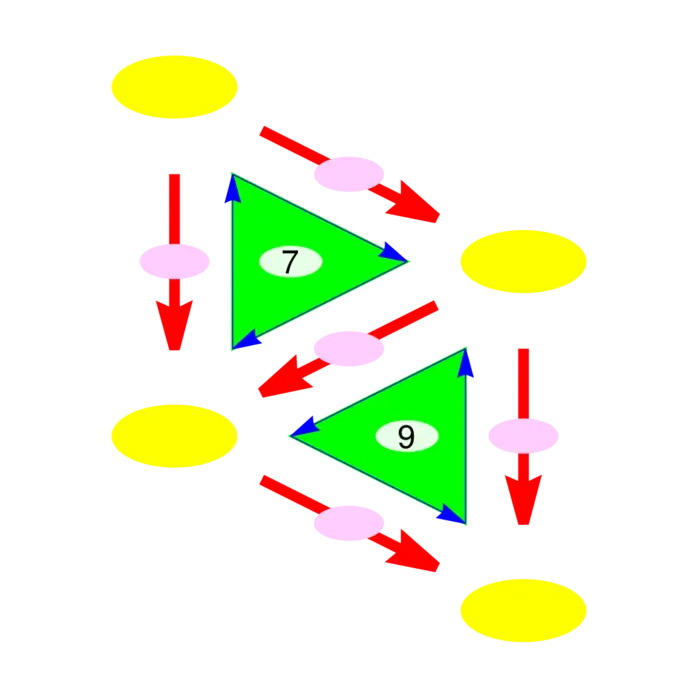
- Given the \(1\)-form \(F\) in Figure (36.4b), compute the \(2\)-form \(d F\).
- Given the \(2\)-form \(H\) in Figure (36.4c), find a \(1\)-form \(F\) such that \(d F=H\). In classical terms, we look for a vector field \(F\) such that \(\operatorname{curl}(F)\) is a given scalar field \(f\) (Classically this is done by solving \(Q_{x}-P_{y}=f\) with \[F=\Big[0, \int_{0}^{x} f(t) \,d t\Big]^{T}\] for example.)
Exercise 3. Given the \(0\)-form \(f\) in Figure (36.4d), check that this \(f\) satisfies \(K f=\lambda f\) for some constant \(\lambda\). This is called an eigenvalue of \(K\).
Exercise 4. Write down the \(4 \times 4\) Kirchhoff matrix \(K\) for the Gaia world. What are the eigenvalues and eigenvectors of \(K\)?
Exercise 5.
- The complete graph with \(4\) elements is the smallest \(3\)-dimensional "world". Find the Kirchhoff Matrix \(K\) of this graph and compute its eigenvalues and eigenvectors. You can use the first line of the Mathematica code below, which computes the Kirchhoff matrix of an other graph and then its Schroedinger evolution.
- If \(\psi\) is an eigenvector of \(K\) satisfying \(K \psi=\lambda \psi\). Verify that \(\psi(t)=e^{-i t \lambda / \hbar} \psi\) solves the Schrödinger equation \(i \hbar \psi^{\prime}=K \psi\). Use a formula seen earlier in this course to explain why quantum mechanics is called "wave mechanics".
SOME LINEAR ALGEBRA
36.6.2 Gaia’s Geometry
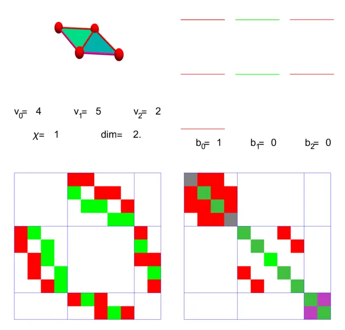
On Gaia, the space of \(0\)-forms is \(4\)-dimensional, the space of \(1\)-forms is \(5\)-dimensional and the space of \(2\)-forms is \(2\)-dimensional.

36.6.3 Gradients, Curls, and Connectivity
We see the Dirac matrix \(D=d+d^{*}\) to the left and the Laplacian \[L=D^{2}=d d^{*}+d^{*} d\] to the right. The first \(4\) columns contain the block \(d_{0}: \Lambda^{0} \rightarrow \Lambda^{1}\) which is the gradient, the top block in the middle \(5\) columns is \(d_{0}^{*}\), the divergence. The bottom block is \(d_{1}: \Lambda_{1} \rightarrow \Lambda_{2}\) the curl. The block in the last \(2\) columns is \(d_{1}^{*}: \Lambda^{2} \rightarrow \Lambda^{1}\) each of the triangles affects \(3\) adjacent edges. The number \(b_{0}\) is the dimension of the kernel of \(L_{0}\). It is called the \(0\)-th Betti number and counts the number of connectivity components of \(G\) (we don’t have a multi-verse), the number \(b_{1}\) is the number of "holes", there are none. Gaia is simply connected.
36.6.4 From Gradients to Kirchhoff
The gradient \(d\) is a matrix which maps a function on vertices to a function on edges. It is a \(|E| \times|V|\) matrix. In Mathematica, you can get \(d^{*}\) with "Incidence matrix". Note that Mathematica distinguishes between directed and undirected graphs and that the gradient is the transpose of \(d\). To compute the Kirchhoffmatrix \(K\), you have to use the undirected graph. Then \(K=d^{*} d\). Here is an example verifying \(K=d^{*} d= \operatorname{divgrad}\).