Dirac Delta Function

A. Dirac Delta Function

[Let us introduce a quantity 𝛿(x), which depends on x satisfying the following conditions:] \[ \delta(x)=0, x\neq 0 \text{, and is in some way infinite for } x=0 \] with \[ \int_{-\infty}^\infty \delta(x)dx = \int_{-\epsilon}^\epsilon \delta(x)dx=1 \] [This quantity is called the Dirac Delta function and is quite useful in physics. We can show that] \[ \int_{-\infty}^\infty f(x)\delta(x)dx = f(0) \]

Proof: \[ \int_{-\infty}^{-\epsilon}f(x)\delta(x)dx + \int_{-\epsilon}^\epsilon f(x)\delta(x)dx + \int_\epsilon^\infty f(x)\delta(x)dx \] If f(x) varies relatively slowly in the range \(-\epsilon\) to \(\epsilon\) we can replace it by an average of f(x) over that interval. \[ \int_{-\infty}^\infty f(x)\delta(x)dx = \int_{-\epsilon}^\epsilon \overline{f(x)}\delta(x)dx \] Letting \(\epsilon\to 0\), we get \[ \begin{aligned} &= \left.\overline{f(x)}\right|_{x\to 0}\int_{-\epsilon}^\epsilon \delta(x)dx\\ &=f(0) \end{aligned} \]

The delta function is useful since it may be operated on as though it were a real function. The only justification we give for this is that it gives the correct answer. \[ f'(t) = -\int_{-\infty}^\infty f(x)\delta'(x-t)dx \] \[ = -f(x)\delta(x-t)\bigg|_{-\infty}^\infty + \int_{-\infty}^\infty f'(x)\delta(x-t)dx \] \[ = 0+f'(t) \] The following useful relations may be easily proved:

\(\delta(x)=\delta(-x)\)
\(\delta'(x)=-\delta'(-x)\)
\(x\delta(x)=0\)
\(x\delta'(x)=-\delta(x)\)
\(\delta(ax) = \dfrac{1}{|a|}\delta(x)\)
\(f(x)\delta(x-a)=f(a)\delta(x-a)\)

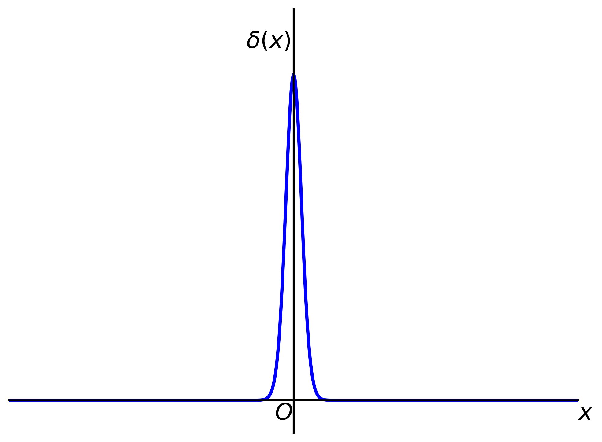
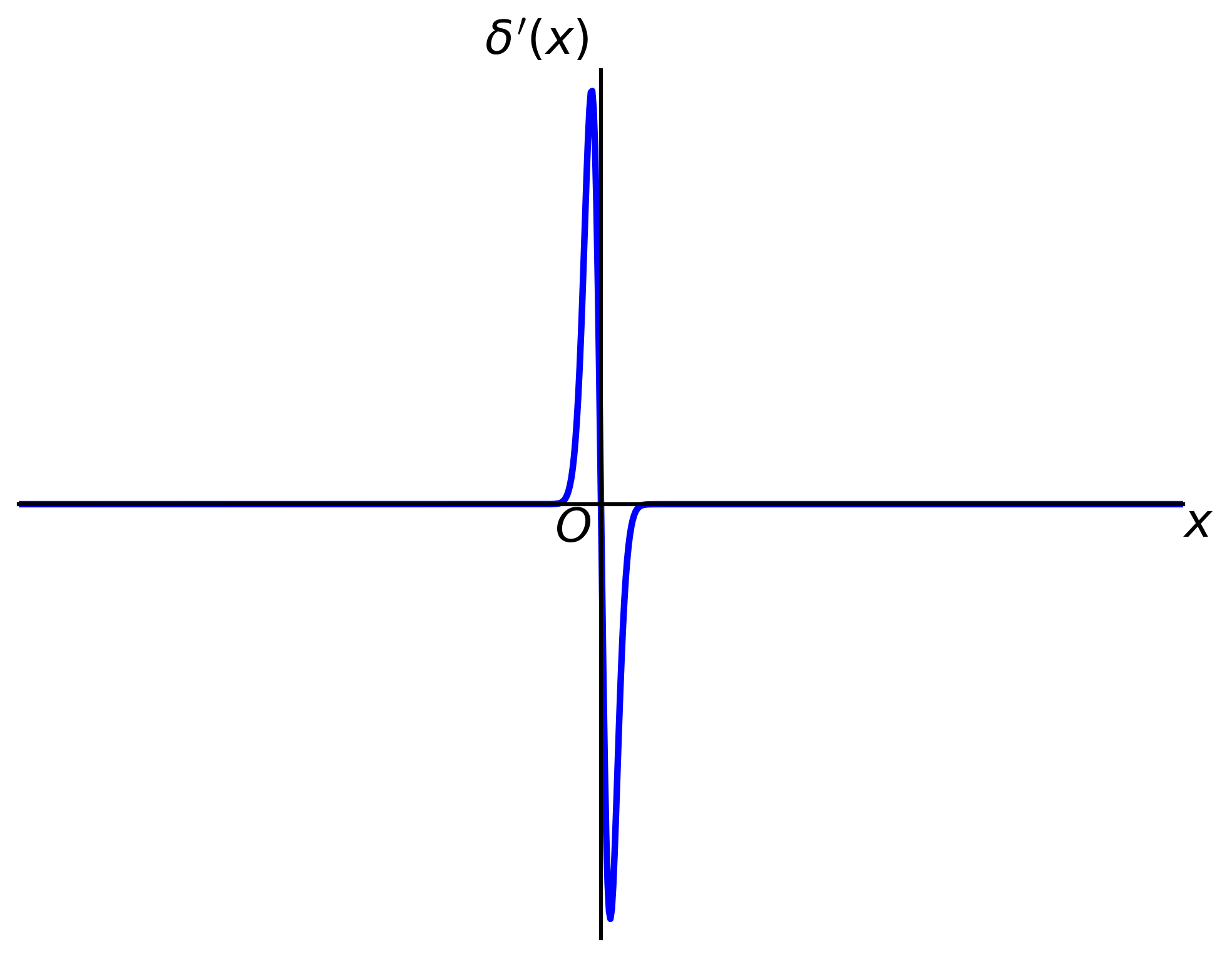
The following figures are approximate representations of \(\delta(x)\) and \(\delta'(x)\).

A diagram shows a sharp peak for δ(x) at x=0

A diagram shows a sharp positive peak followed by a sharp negative peak for δ'(x) at x=0

Problem: (with integrals)

Prove: \(\delta(ax)=\dfrac{1}{a}\delta(x)\) for \(a>0\)
Find: \(x\delta''(x)=?\)

B. Step Function

\[ \int_{-\infty}^x \delta(t)dt = \begin{cases} 0 & x<0 \\ 1 & x>0 \end{cases} \]

Explanation

The function being described on the right-hand side is the Heaviside step function, often written as H(x) or θ(x)

Case 1 (x<0) The integral’s upper limit x is negative. The integration range is from −∞ to x. This range does not include t=0 where the delta functon is non-zero. Therefore, you are integrating a function that is zero over the entire interval, and the result is 0.
Case 2 (x>0): The integral’s upper limit x is positive. The integration range from −∞ to xdoes include t=0. Because the entire “spike” of the delta function is included in the range, the integral evaluates to the total area of the delta function, which is 1.

Notice that \(H^\prime(x)=\delta(x)\).

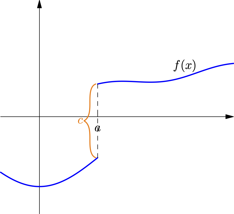
Consider the curve in the following figure. Its derivative may be expressed in terms of the delta function as follows: \[ f'(x) = f'(x)_{x\neq a} + c\delta(x-a) \]

A diagram shows a function f(x) with a step discontinuity of height c at x=a

Explanation

Let’s take any function f(x) that is smooth everywhere except for a single jump discontinuity of height c at x=a.

We can represent this function f(x) as the sum of two parts:

A continuous smooth “base” function, let’s call it g(x).
A step function that adds the jump at the right place.

The formula is: \[ f(x) = g(x) + c \cdot H(x-a) \]

How do we find g(x)? The function g(x) is simply the “pre-jump” part of the function extended across the entire domain.

For x < a, we have H(x-a)=0, so f(x) = g(x). This means g(x) is identical to f(x) before the jump.
For x > a, we have H(x-a)=1, so f(x) = g(x) + c. This correctly describes the function after the jump.

Differentiating the Representation

Now that we have expressed f(x) in a form that is a sum of well-behaved functions (a continuous function and a Heaviside function), we can differentiate it using the sum rule: \[ f'(x) = \frac{d}{dx} \left[ g(x) + c \cdot H(x-a) \right] \] \[ f'(x) = \frac{d}{dx} g(x) + c \cdot \frac{d}{dx} H(x-a) \]

Using the relationship \(\frac{d}{dx}H(x-a) = \delta(x-a)\), we get: \[ f'(x) = g'(x) + c \cdot \delta(x-a) \]

Now, what is g’(x)? Since g(x) is the continuous version of f(x), its derivative g’(x) is exactly the same as the derivative of f(x) away from the jump, i.e., for \(x \neq a\).

So, we can replace g’(x) with the notation f’(x)_{x a} to get the final formula: \[ f'(x) = f'(x)_{x\neq a} + c \cdot \delta(x-a). \]

C. Delta function and the integral of cos(ßx)

Consider the integral: \(\displaystyle \int_{-\infty}^\infty \cos \beta x\, dx\). We shall show that it is equal to \(2\pi\delta(\beta)\). \[ \int_0^{\infty} \cos\beta x\, dx = \pi\delta(\beta). \]

Explanation

Notice that \(\int_0^\infty\) cos(ßx) dx does not converge in the usual sense because the cosine function oscillates forever. To give it a meaningful value, we treat it as a distribution by examining its behavior in a limit.

\[ \lim_{a\to 0} \int_0^\infty e^{-ax}\cos\beta x\, dx = \lim_{a\to 0} \dfrac{a}{a^2+\beta^2} \]

Explanation

It was previously shown that \[ \int_0^\infty e^{-ax}\cos(\beta x) dx=\frac{a}{a^2+\beta^2} \]

For small \(a\) this integral looks approximately as in the following figure.

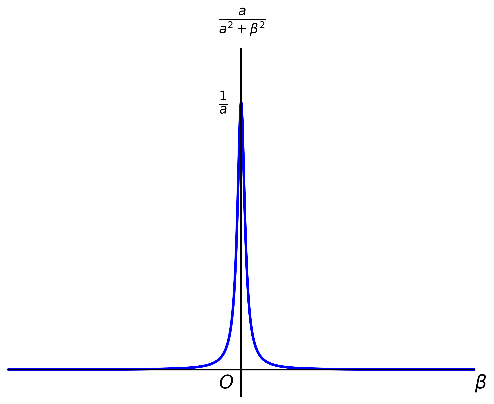
A diagram shows a bell-shaped curve centered at ß = 0 with height 1/a

The area under the curve is: \[ A = \int_{-\infty}^\infty \left(\dfrac{a}{a^2+\beta^2}\right)d\beta = \int_{-\infty}^\infty \dfrac{a^2}{a^2+a^2z^2}dz \] \[ = \int_{-\infty}^\infty \dfrac{dz}{1+z^2} = \left. \tan^{-1}z \right|_{-\infty}^\infty = \pi \] Note that the area is independent of the value of a.

Explanation

The function \(\frac{a}{a^2+\beta^2}\) has an area of π for any value of a. As a→0, the function becomes an infinitely thin, infinitely high spike at β=0, while its total area remains π. This is precisely the behavior of πδ(β).

D. Use of the delta function in evaluating a definite integral

Example: Consider \[ \int_0^\pi \cos(m\tan\theta)d\theta \] Substitute \(\tan\theta = x\) \[ \int_0^\infty \cos mx(1+x^2)^{-1}dx = S(m) \] \[ -\int_0^\infty x^2 \cos(mx)(1+x^2)^{-1}\, dx=S''(m) \] \[ S(m)-S''(m) = \int_0^\infty \cos mx\ dx = \pi\delta(m) \] The general solution of such a differential equation is: \[ S(m) = \dfrac{e^{-m}}{2}\int_{-\infty}^m e^{-t} f(t)dt - \dfrac{e^m}{2}\int_{-\infty}^m e^{t}f(t)dt + Ae^m+Be^{-m} \] where \(f(t) = \pi\delta(t)\)

Explanation

From differential equations, recall that if \(y_1(x)\) and \(y_2(x)\) are two solutions the equation \(y''+P(x)y'+Q(x)=0\), then a particular solution of \(y''+P(x)y'+Q(x)=R(x)\) is given by \[ -y_1(x)\int_{x_0}^x \frac{y_2(t)R(t)}{W(t)}dt+y_2(x)\int_{x_0}^x \frac{y_1(t)R(t)}{W(t)}dt \] where \(W(t)=W[y_1(t),y_2(t)]\) is the Wronskian.

For the equation \(S''(m)-S(m)=0\), we look for solutions of the form \(e^{rm}\). The characteristic equation is \(r^2-1=0\), which has roots \(r=\pm 1\). This gives us two independent solutions of the corresponding homogeneous equation: \[ S_1(m)=e^{m},\qquad S_2(m)=e^{-m}. \] The homogeneous solution is \[ S_h(m)=A S_1(m)+B S_2(m)=A e^m+B e^{-m}. \] The Wronskian is \[ \begin{vmatrix} S_1(m) & S_2(m)\\ S_1^\prime(m) & S_2^\prime(m) \end{vmatrix}=\begin{vmatrix} e^m & e^{-m}\\ e^m & -e^{-m} \end{vmatrix}=-1-1=-2. \] According to the theorem mentioned above, a particular solution is given by \[ S_p(m)=e^m \int_{-\infty}^m \frac{e^{-t}f(t)}{-2} dt-e^{-m}\int_{-\infty}^m \frac{e^t f(t)}{-2}dt \] and the total solution is \[ S(m)=S_h(m)+S_p(m) \]

Solutions: \[ \begin{aligned} m<0 \quad &S=Ae^m+Be^{-m}\\ m>0 \quad &S=Ae^m+Be^{-m}-\dfrac{\pi}{2}e^m+\dfrac{\pi}{2}e^{-m} \end{aligned} \]

Explanation

Previously, we obtained \[ S_p(m)=\frac{\pi}{2}e^{-m}\int_{-\infty}^m \delta(t) e^{-t}dt-\frac{\pi}{2} e^m\int_{-\infty}^m \delta(t)e^{-t} dt \] If \(m<0\): \[ S_p(m)=0 \]and the total solution is \[ S(m)=A e^m+B e^{-m} \] If \(m>0\) then \[ S_p(m)=\frac{\pi}{2}e^{-m}e^0-\frac{\pi}{2}e^m e^0 \] and the total solution is \[ S(m)=A e^m+B e^{-m}+\frac{\pi}{2} e^{-m}-\frac{\pi}{2}e^m \]

\[ S(0) = \dfrac{\pi}{2} = A+B \] \[ S(m)=S(-m)\quad \therefore A-B=\dfrac{\pi}{2} \] \[A=\dfrac{\pi}{2}, B=0 \] \[m<0 \quad S=\dfrac{\pi}{2}e^m\] \[ m>0 \quad S=\dfrac{\pi}{2}e^{-m} \]

Example: Let us consider the integral \[ \int_{-\infty}^\infty \dfrac{\sin\beta x}{x}dx = S(\beta) \] [If we differentiate with respect to \(\beta\), we get the \(\int_0^\infty \cos \beta x dx\) where we know is \(2\pi \delta(\beta)\):] \[ S'(\beta) = \int_{-\infty}^\infty x\dfrac{\cos\beta x}{x} dx= 2\pi\delta(\beta) \] [Solving this differential equation, we get:] \[ \begin{aligned} S(\beta) &= 2\pi+C \quad \beta>0 \\ S(\beta) &= C \quad \beta<0 \end{aligned} \] We note that \(S(\beta) = -S(-\beta)\) \[ 2\pi+C = -C \] \[ C=-\pi \] \[ \begin{aligned} \beta>0 \quad S(\beta) = \pi \\ \beta<0 \quad S(\beta) = -\pi \end{aligned} \] (A graph shows a step function, going from -π for β<0 to +π for β>0)

Consider now the integral \[ \int_0^\infty e^{-\alpha x}\dfrac{\sin\beta x}{x}dx = \dfrac{\pi}{2}-\tan^{-1}(\alpha/\beta) \]

Explanation

Notice that we previously studied this integral.

A graph of this integral looks as follows:

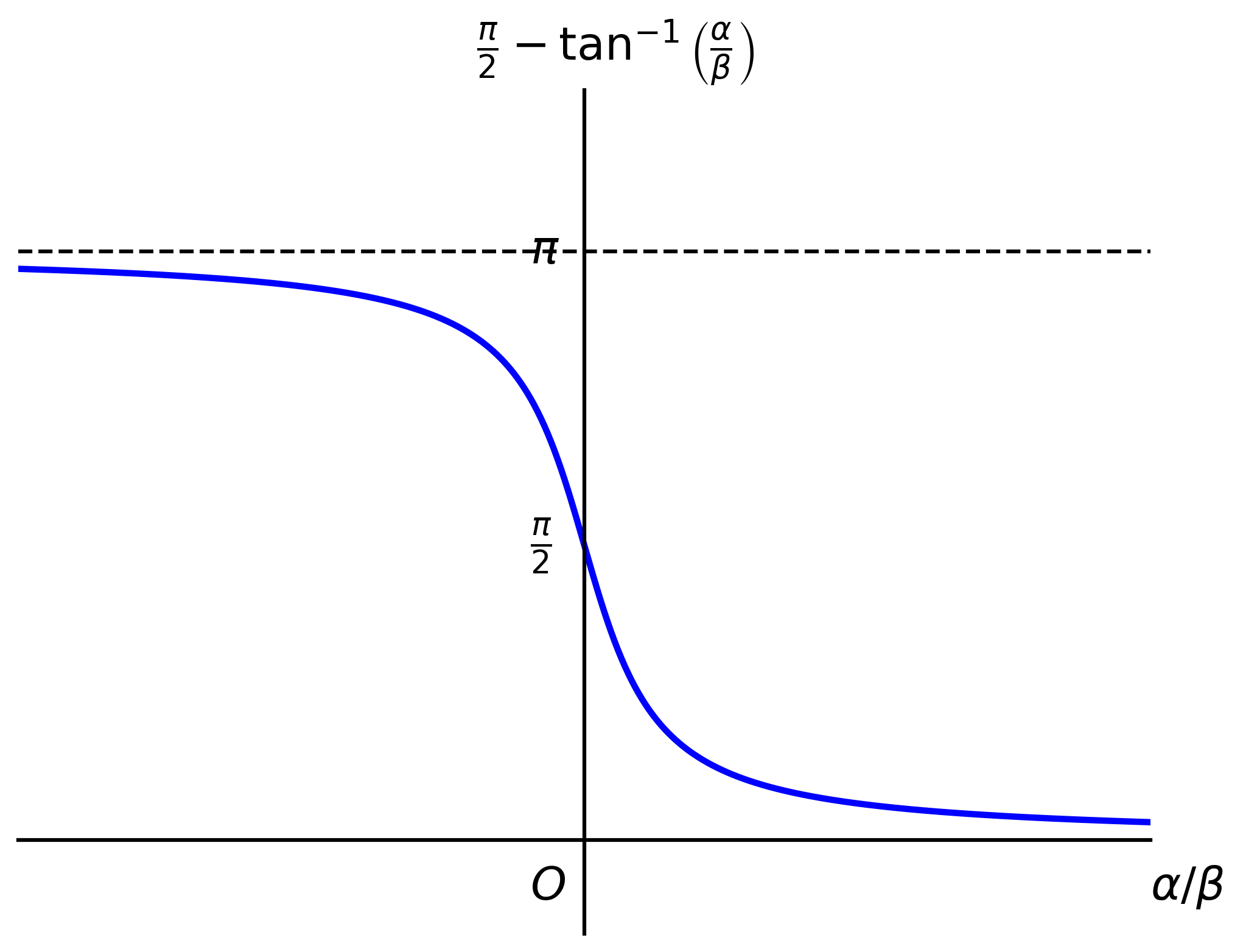
In the lim \(\alpha\to 0\), this integral reduces to the one considered previous to it (there is a factor 2 to be considered)

Reference: Principals of Quantum Mechanics, Paul Dirac, 4th ed., p. 58–61