We intuitively say that a variable is a function of a second variable when its value depends on the value of the second variable and the value of the first variable can be uniquely calculated by some rule when the value of the second variable is assumed. The first variable is called the dependent variable and the second the independent variable .
Read some examples
For example, the temperature at which pure water boils is a function of the altitude above sea level. The area of a circle \(A\) is a function of its radius \(r\) , because if the radius of a circle \(r\) is given, we can calculate its area \(A=\pi r^{2}\) . Thus the area is a function of the radius. Conversely, if the area of a circle is given, we can calculate its radius through \(r=\sqrt{A/\pi}\) . Thus, the radius is a function of the area. Sometimes, like in this example, it is a matter of choice which variable is called the independent variable and which one the dependent variable.
In a triangle, suppose the lengths of two sides, \(a\) and \(b\) , are given. If we choose a value between 0 and 180 \(^{\circ}\) for the angle \(\gamma\) between these two sides, then the length of the third side \(c\) is determined. Thus if \(a\) and \(b\) are given, we can say \(c\) is a function of \(\gamma\) . From geometry we know that this function is represented by the formula \[c=\sqrt{a^{2}+b^{2}-2ab\cos\gamma}.\]
The federal tax rate for a single person is a function of his or her taxable income. For example, if his or her taxable income is any number between $38,701 and $82,500, the tax rate is 22% and if the taxable income is between $9,526 and $38,700, the tax rate falls into 12%.
- A variable can be a function of more than one other variable. For example, the volume of a circular cylinder \(V\) is a function of the radius of its base \(r\) and the height of the cylinder \(h\) . We need to know both \(r\) and \(h\) to be able to calculate \(V\) through \(V=\pi r^{2}h\) . We will study multivariable functions only in the second part of the course.
The formula \(y=\sqrt{x}\) defines \(y\) as a function of \(x\) for nonnegative values of \(x\) , as square roots of negative numbers are undefined. In the equation \(y=x^{2}\) , \(y\) is a function of \(x\) because each value of \(x\) yields a unique \(y\) ; however, \(x\) is not a function of \(y\) because a positive \(y\) corresponds to two values of \(x\) (except when \(y=0\) ).
The formula \[y=\sqrt{x},\] defines \(y\) as a function of \(x\) for all \(x\geq0\) (we restrict the values of \(x\) to nonnegative numbers because we cannot take the square root of a negative number).
If \(x\) and \(y\) are two variables connected by the relation \[y=x^{2},\] then \(y\) is a function of \(x\) because if the value of \(x\) is given, the value of \(y\) can be calculated uniquely. Conversely if the value of \(y>0\) is given (for example \(y=4\) ), this equation defines two corresponding values of \(x\) (for example, \(x=+2\) or \(x=-2\) corresponding to \(y=4\) ). Because not a unique value of \(x\) corresponds to a given value of \(y\) (except when \(y=0\) ), \(x\) is not a function of \(y\) .
In mathematics, to denote that \(y\) is a function of \(x\) , we use the notation \(y=f(x)\) , where \(f\) symbolizes the rule associating \(x\) values with \(y\) values, and various symbols like \(g(x)\) , \(\phi(x)\) , \(F(x)\) , etc., are used to represent different functions.
In mathematics, we often wish to refer to a generic function without specifying any particular formula, table, or graph. To denote that \(y\) is a function of \(x\) , we write \[y=f(x),\] which is read as “ \(y\) is equal to \(f\) of \(x\) .” In this notation, \(f\) represents the function, that is, the “rule” or “procedure” (which usually but not always involves some formula) associating the values of \(x\) to the values of \(y\) . Instead of \(f(x)\) , we may use other notations such as \(g(x)\) , \(\phi(x)\) , \(F(x)\) , \(f'(x)\) , \(s(x)\) , etc. If more than a function occur in a problem, one may be expressed as \(f(x)\) , another as \(F(x)\) , another as \(g(x)\) , and so on. It is also convenient in practice to represent different functions by the symbols \(f_{1}(x),f_{2}(x),f_{3}(x)\) , etc. However, during any investigation, the same functional symbol always indicates the same law of dependence of the dependent variable upon the independent variable.
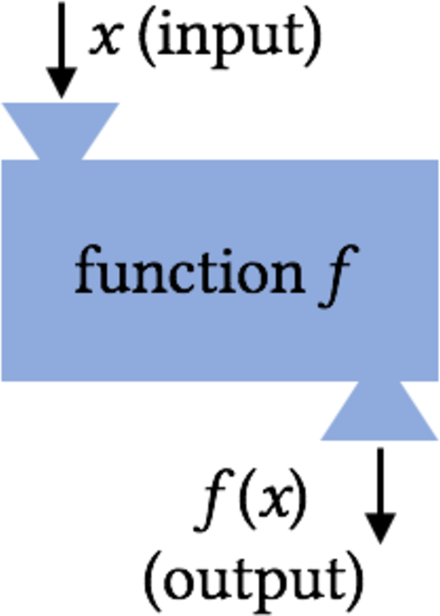
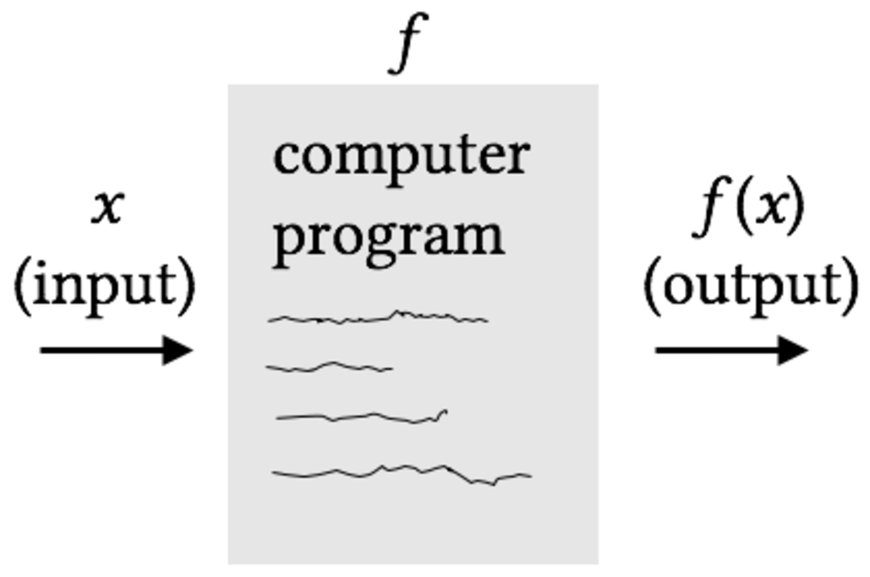
A function can be thought of as a machine or a computer program that assigns one output to every allowable input.
 |
| (a) |
 |
| (b) |
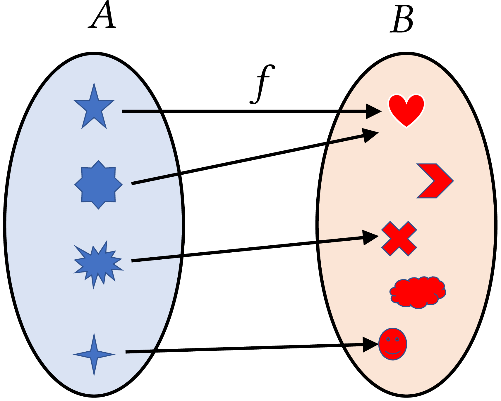
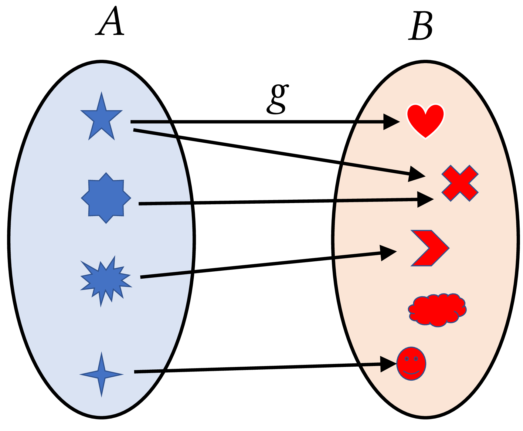
Another way to picture a function is by an arrow diagram. For each element \(x\) in \(A\) , the value of \(f(x)\) in \(B\) is to be found at the head of the corresponding arrow. As we can see in the following figure (a), \(f\) associates to each element in \(A\) , one and only one element in \(B\) . Thus, \(f\) is a function, although two elements in \(A\) are associated with one element (heart) in \(B\) . But in the following figure (b), \(g\) associates two elements to an element (star) in \(A\) . Therefore, \(g\) is not a function.
 |
| (a) |
 |
| (b) |
Definition 5.1 . A function \(f\) from a set \(A\) , to a set \(B\) , is a rule that assigns, to each element \(x\) in \(A\) , one and only one element \(y\) in \(B\) . We then write \(y=f(x)\) .
Sets \(A\) and \(B\) are called domain and co-domain of \(f\) , respectively. To mention that \(f\) is a function with domain \(A\) and co-domain \(B\) , we write \(f:A\rightarrow B\) .
- If \(y=f(x)\) , we also call the independent variable \(x\) , the argument of the function, and the element \(y\) the value of \(\boldsymbol{f}\) at \(\boldsymbol{x}\) or the image of \(\boldsymbol{x}\) under \(\boldsymbol{f}\) .
- The definition of a function \(f:A\to B\) does not restrict the nature of the elements of \(A\) and \(B\) , but in elementary calculus we assume that they are numbers; that is, \(A\) and \(B\) are subsets of real numbers \(\mathbb{R}\) , unless otherwise stated.
If \(y=f(x)\) , the particular value of the function when \(x\) has a definite value \(a\) is then expressed as \(f(a)\) .
Example 1. If \(f(x)=4x^{2}-5x+1\) , find
\(f(-1)\) , \(f(0)\) , \(f(t)\) , \(f(u)\) , \(f(b+1)\) , and \(f(x+h)\) .
Solution
If \[f(x)=4x^{2}-5x+1,\] then \[f(-1)=4(-1)^{2}-5(-1)+1=10,\] and \[f(0)=4(0)^{2}-5(0)+1=1.\] Also, because it does not matter which letter we use for the independent variable, we have \[f(t)=4t^{2}-5t+1,\] \[f(u)=4u^{2}-5u+1,\] \[f(b+1)=4(b+1)^{2}-5(b+1)+1=4b^{2}+3b,\] and \[\begin{align} f(x+h)&=4(x+h)^2-5(x+h)+1\\ &=4(x^2+2xh+h^2)-5x-5h+1\\ &=\underbrace{4x^2-5x+1}_{f(x)}+8xh-5h+4h^2. \end{align}\]
Strictly speaking \(f(x)\) is the value of \(f\) at \(x\) , but we often talk about “the function \(f(x)\) ” or “the function \(y=f(x)\) .” For example, consider a function \(f:\mathbb{R}\to\mathbb{R}\) that takes a number \(x\) and gives its square \(x^{2}\) . In this case, we can simply say:
- “the function \(f(x)=x^{2}\) ;”
- “the function \(y=x^{2}\) ” (if we denote the dependent variable by \(y\) );
- or even simply “the function \(x^{2}\) .”
We can also connect the input and output values by a special arrow, namely “the function \(x\mapsto x^{2}\) .”
Table of Contents
Implicit and Explicit Functions
Functions can be categorized as either explicit or implicit, each with distinct characteristics:
- Explicit Function : An explicit function clearly expresses the dependent variable in terms of the independent variable(s). The most common form is \(y = f(x)\) , where \(y\) is directly given as a function of \(x\) . For example, \(y = x^2 + 3\) is the equation of an explicit function because \(y\) is directly expressed in terms of \(x\) .
- Implicit Function : An implicit function, on the other hand, involves an equation where the dependent and independent variables are intermixed, and the dependent variable is not explicitly isolated. For example, in the equation \(x^2 + y^2 = 1\) or \(x^3-3xy+y^3=0\) , \(y\) is not explicitly solved for in terms of \(x\) ; instead, both \(x\) and \(y\) are part of a relationship that defines \(y\) implicitly. The notation \(f(x,y)=0\) is used to denote that \(x\) and \(y\) are implicit functions of each other.
In this book, we almost always work with explicit functions. This trend largely continues into calculus, where implicit functions are encountered relatively infrequent.