Every formula in this chapter comes from the same idea: write down the infinitesimal element of the quantity you want, then integrate it. Learn the method and you can rebuild any of the formulas from scratch.
In the previous chapters we approximated the net area under the curve by dividing the interval of into small subintervals and forming Riemann sums. As the maximum length of the subintervals goes to zero (and the number of subintervals goes to infinity), these sums approach a limit equal to the exact area. We then learned how to calculate that limit with the Fundamental Theorem of Calculus. In fact, that entire development can be summarized in a single line:
\begin{aligned} \lim_{\max\Delta_{k}x\to0}\sum_{k=1}^{n}f(x_{k}^{*})\,\Delta_{k}x &=\int_{a}^{b}f(x)\,dx\\ &=F(x)\bigg|_{x=a}^{x=b}=F(b)-F(a), \end{aligned}where is an antiderivative of .
Many other quantities, the volume and surface area of a solid, the length of a curve, the work done by a variable force, can be calculated by essentially the same process. We divide the interval of the independent variable into small pieces, form the corresponding sums to approximate the quantity, and then take the limit of those sums. That limit is the exact value of the quantity.
The Element Method
Once the limit-of-sums process is understood, we do not have to rebuild every detail for each new quantity. Instead we take an intuitive shortcut and write down the formulas directly.
Look once more at the area formula
since . We can imagine that (or ) is the area of a rectangle of base and height , located at a position specified by a value of x between a and b. The area of this infinitesimal rectangle, denoted , is called the differential element of area, or simply the element of area:
Now we conceive the required area as the result of adding up these differential elements as the rectangle sweeps across the region. Symbolically,

In this practical way of thinking we skipped the laborious details, dividing the region into rectangles of base and height , forming the sums, taking the limit, and then switching to , to , and to , and went directly to the formula for the area under a curve. This intuitive approach to integration is used constantly in science and engineering.
- Note that if denotes the area under the graph of between and , then
The Fundamental Theorem of Calculus asserts that
This is exactly what we wrote for the differential element of area, so the shortcut is not a fudge: the Fundamental Theorem is what licenses it.
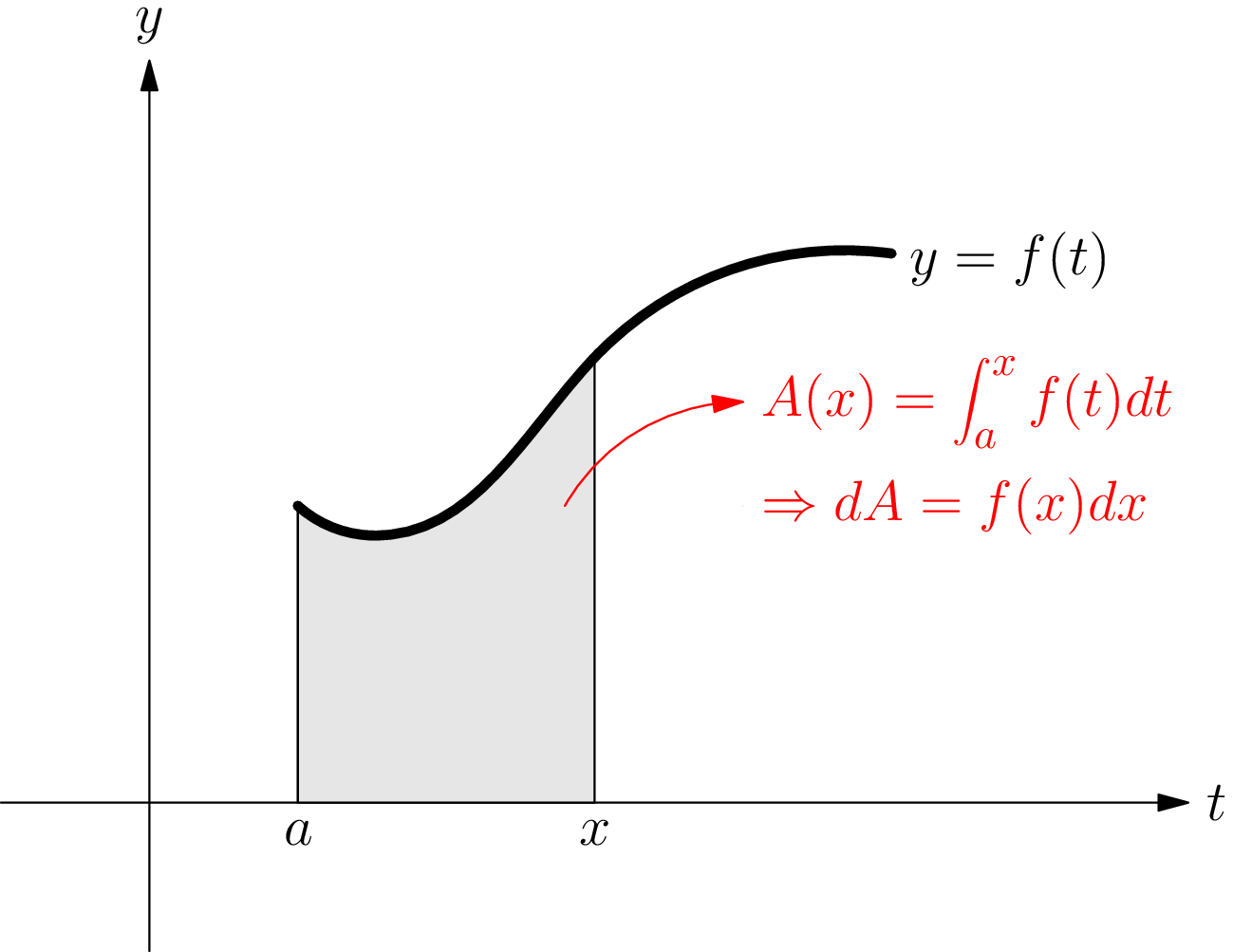
is the area under the graph of between the fixed endpoint and the variable point .

In this chapter, try to understand the method we use to construct the formulas rather than just memorizing the formulas. If you understand the method, you can construct any of them from scratch whenever you need one.
Sections in This Chapter
| Section | Topic | Element | Formula |
|---|---|---|---|
| 8.1 | The Area Between Two Curves | Thin rectangle | |
| 8.2 | Volumes of Solids of Revolution: The Disk and Washer Methods | Thin disk or washer | , |
| 8.3 | Volumes of Solids With Known Cross Sections: The Slice Method | Thin slice | |
| 8.4 | Volumes: The Shell Method | Thin cylindrical shell | |
| 8.5 | Arc Length | Short piece of curve | |
| 8.6 | Areas of Surfaces of Revolution | Thin collar | |
| 8.7 | Work | Small displacement |
Read the sections in order. Section 8.1 establishes the pattern with the quantity you already understand, area. Sections 8.2 through 8.4 give three different ways of slicing the same kind of solid, and part of the skill is choosing the one that makes the integral easiest. Section 8.5 introduces the arc length element , which Section 8.6 immediately reuses to build surfaces. Section 8.7 leaves geometry behind and applies the identical reasoning to a physical quantity.
Where These Ideas Are Used
- Manufacturing and machining. Pistons, axles, funnels, bottles, and turned wooden and metal parts are solids of revolution. Their volume, and therefore their mass and material cost, is a disk, washer, or shell integral.
- Civil and structural engineering. The volume of earth to be moved for a cutting or an embankment is a slice integral over cross sections surveyed at regular intervals along the route.
- Naval architecture. A ship's displacement is computed by integrating the area of its cross sections, and its wetted surface area, which determines drag, is a surface-of-revolution-style integral.
- Architecture and design. Domes, vases, columns, and cooling towers are generated by revolving a profile curve, a construction studied by Renaissance draughtsmen such as Paolo Uccello long before calculus existed.
- Roads, cables, and pipelines. The length of a suspension cable hanging in a catenary, or of a road following a curved profile, is an arc length integral, and it determines how much material to order.
- Coating, painting, and heat transfer. The amount of paint or plating needed for a turned surface, and the rate at which a body loses heat, are both proportional to surface area.
- Mechanics and hydraulics. The work done stretching a spring, lifting a hanging chain, pumping a tank empty, or moving a mass out of a gravitational field is a work integral .
- Thermodynamics. The work done by an expanding gas is , which is the same integral wearing different symbols.
A Word on Method
Almost every problem in this chapter yields to the same four steps.
- Draw the picture. Sketch the region or the solid, and mark the axis of revolution if there is one. Most errors in this chapter are geometric, not algebraic.
- Draw one typical element and label its dimensions: a rectangle of width or , a disk of radius and thickness , a shell of radius and height , a layer of liquid of thickness lifted a distance .
- Write the element of area, volume, length, surface, or work in terms of a single variable. If two variables appear, use the equation of the curve to eliminate one.
- Find the limits and integrate. The limits are the extreme positions of the element as it sweeps through the whole region, which is usually where two curves intersect.
Whenever the answer can be checked against elementary geometry, a cone, a sphere, a cylinder, do the check. It costs a line and catches most mistakes.
